Practical 5: Numerical approaches

Introduction

In previous practicals you have used Bayesian models with conjugate priors where the posterior distribution can be easily worked out. In general, this is seldom the case and other approaches need to be considered. In particular, Importance Sampling and Markov Chain Monte Carlo (MCMC) methods can be used to draw samples from the posterior distribution that are in turn used to obtain estimates of the posterior mean and variance and other quantities of interest.

Importance Sampling

As described in the previous lecture, Importance Sampling (IS) is an algorithm to estimate some quantities of interest of a target distribution by sampling from a different (proposal) distribution and reweighting the samples using importance weights. In Bayesian inference, IS can be used to sample from the posterior distribution when the normalizing constant is not known because $\pi(\theta \mid \mathbf{y}) \propto L(\theta \mid \mathbf{y}) \pi(\theta),$ where $\mathbf{y}$ represents the observed data, $L(\theta \mid \mathbf{y})$ the likelihood function and $\pi(\theta)$ the prior distribution on $\theta$ .

If $g(\cdot)$ is a proposal distribution, and $\{\theta^{(m)}\}_{m=1}^M$ are $M$ samples from that distribution, then the importance weights are $w(\theta^{(m)}) = \frac{L(\theta^{(m)} \mid \mathbf{y})\,\pi(\theta^{(m)})} {g(\theta^{(m)})} .$ When the normalising constant in the posterior distribution is not known, the importance weights are rescaled to sum to one. Note that this rescaling is done by the denominator in the expression at point 2 on slide 14/30 of the Numerical Approaches slides you have just seen. In practice, rescaling removes the need for the denominator and simplifies the calculations throughout (we do it once, rather than every time).

Hence, the posterior mean can be computed as $E\left(\theta \mid \mathbf{y}\right) = \mu = \int \theta\, \pi(\theta \mid \mathbf{y}) \mathop{d\theta} \simeq \sum_{m=1}^M \theta^{(m)}\, w(\theta^{(m)}) = \hat{\mu}.$ Similarly, the posterior variance can be computed as $\mbox{Var}\left(\theta \mid \mathbf{y}\right) = \sigma^2 = \int (\theta - \mu)^2\, \pi(\theta \mid \mathbf{y}) \mathop{d\theta} \simeq \sum_{m=1}^M (\theta^{(m)})^2\, w(\theta^{(m)}) - \hat{\mu}^2 .$

The Metropolis-Hastings Algorithm

The Metropolis-Hastings (M-H) algorithm is a popular MCMC method to obtain samples from the posterior distribution of an ensemble of parameters. In the example below we will only consider models with one parameter, but the M-H algorithm can be used on models with a large number of parameters.

The M-H algorithm works in a very simple way. At every step of the algorithm a new movement is proposed using a proposal distribution. This movement is accepted with a known probability, which implies that the movement can be rejected so that the algorithm stays at the same state in the current iteration.

Hence, in order to code the M-H algorithm for a set of parameters $\theta$ we need to define:

A function to draw observations from the proposal distribution, given its current state. This will be denoted by $q(\cdot\mid\cdot)$ , so that the density of a new proposal $\theta^*$ given a current state $\theta^{(m)}$ is given by $q(\theta^*\mid\theta^{(m)})$ .

From the Bayesian model, we already know:

A prior distribution on the parameters of interest, i.e., $\pi(\theta)$ .
The likelihood of the parameter $\theta$ given the observed data $\mathbf{y}$ , i.e., $L(\theta\mid\mathbf{y})$ .

At step $m$ , a new value is drawn from $q(\cdot\mid\theta^{(m)})$ and it is accepted with probability:

$\alpha = \min\left\{1, \frac{L(\theta^*\mid\mathbf{y})\,\pi(\theta^{*})\,q(\theta^{(m)} \mid\theta^{*})} {L(\theta^{(m)}\mid\mathbf{y})\,\pi(\theta^{(m)})\,q(\theta^{*} \mid\theta^{(m)})}\right\}$

If the value is accepted, then the current state is set to the proposed value, i.e., $\theta^{(m+1)} = \theta^{*}$ . Otherwise we keep the previous value, so $\theta^{(m+1)} = \theta^{(m)}$ .

Example: Poisson-Gamma Model

The first example will be based on the Game of Thrones data set. Remember that this is made of the observed number of u’s on a page of a book of Game of Thrones. The model can be stated as:

$\begin{array}{rcl} y_i \mid \lambda & \sim & \text{Po}(\lambda)\\ \lambda & \sim & \text{Ga}(\alpha,\, \beta) \end{array}$

In particular, the prior on $\lambda$ will be a Gamma distribution with parameters $0.01$ and $0.01$ , which is centred at 1 and has a small precision (i.e., large variance).

We will denote the observed values by y in the R code. The data collected can be loaded with:

GoTdata <- data.frame(Us = c(25, 29, 27, 27, 25, 27, 22, 26, 27, 29, 23,
                          28, 25, 24, 22, 25, 23, 29, 23, 28, 21, 29,
                          28, 23, 28))
y <- GoTdata$Us

Importance sampling

Now the parameter of interest is not bounded, so the proposal distribution needs to be chosen with care. We will use a log-Normal distribution with mean 3 and standard deviation equal to 0.5 in the log scale. This will ensure that all the sampled values are positive (because $\lambda$ cannot take negative values) and that the sample values are reasonable (i.e., they are not too small or too large). Note that this proposal distribution has been chosen having in mind the problem at hand and that it may not work well with other problems.

n_simulations <- 10000
set.seed(1)
lambda_sim <- rlnorm(n_simulations, 3, 0.5)

Next, importance weights are computed in two steps. First, the ratio between the likelihood times the prior and the density of the proposal distribution is computed. Secondly, weights are re-scaled to sum to one.

# Log-Likelihood (for each value of lambda_sim)
loglik_pois <- sapply(lambda_sim, function(LAMBDA) {
  sum(dpois(GoTdata$Us, LAMBDA, log = TRUE))
})

# Log-weights: log-lik + log-prior - log-proposal_distribution
log_ww <- loglik_pois + dgamma(lambda_sim, 0.01, 0.01, log = TRUE) - dlnorm(lambda_sim, 3, 0.5, log = TRUE)

# Re-scale weights to sum up to one
log_ww <- log_ww - max(log_ww)
ww <- exp(log_ww)
ww <- ww / sum(ww)

The importance weights can be summarized using a histogram:

hist(ww, xlab = "Importance weights")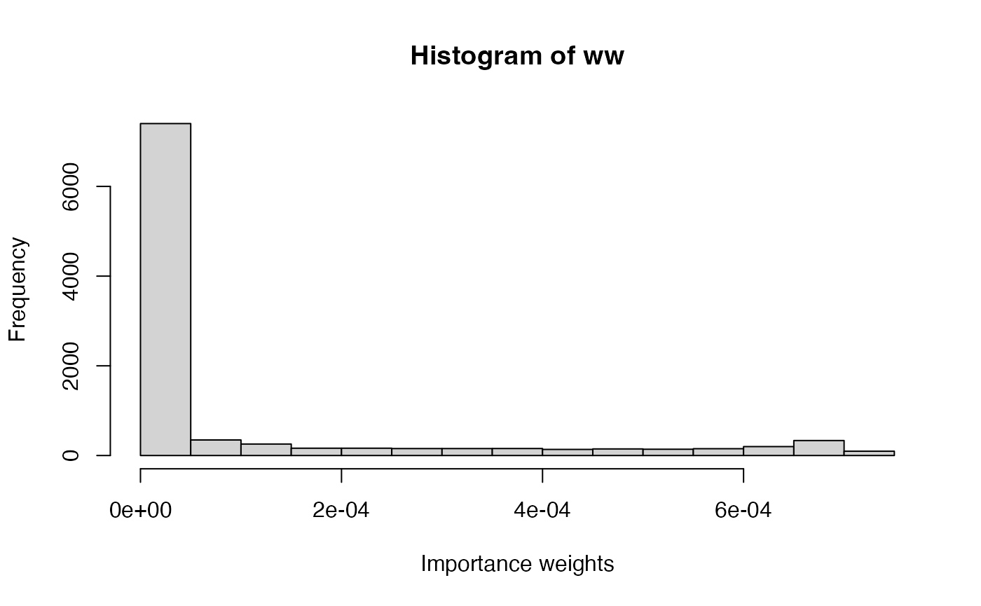

The posterior mean and variance can be computed as follows:

# Posterior mean
(post_mean <- sum(lambda_sim * ww))

## [1] 25.71561

# Posterior variance
(post_var <- sum(lambda_sim^2 * ww)- post_mean^2)

## [1] 0.9987383

Finally, an estimate of the posterior density of the parameter can be obtained by using weighted kernel density estimation.

Aside: weighted kernel density estimation Standard kernel density estimation is a way of producing a non-parametric estimate of the distribution of a continuous quantity given a sample. A kernel function is selected (typically a Normal density), and one of these is placed centred on each sample point. The sum of these functions produces the kernel density estimate (after scaling - dividing by the number of sample points). A weighted kernel density estimate simply includes weights in the sum of the kernel functions. In both weighted and unweighted forms of kernel density estimation, the key parameter controlling the smoothness of the resulting density estimate is the bandwidth (equivalent to the standard deviation if using a Normal kernel function); larger values give smoother density estimates, and smaller values give noisier densities.

plot(density(lambda_sim, weights = ww, bw = 0.5) , main = "Posterior density", xlim = c(10,40))

Note that the value of the bandwidth used (argument bw) has been set manually to provide a realistically smooth density function.

Similarly, a sample from the posterior distribution can be obtained by resampling the original values of $\theta$ with their corresponding weights.

post_lambda_sim <- sample(lambda_sim, prob = ww, replace = TRUE)
hist(post_lambda_sim, freq = FALSE)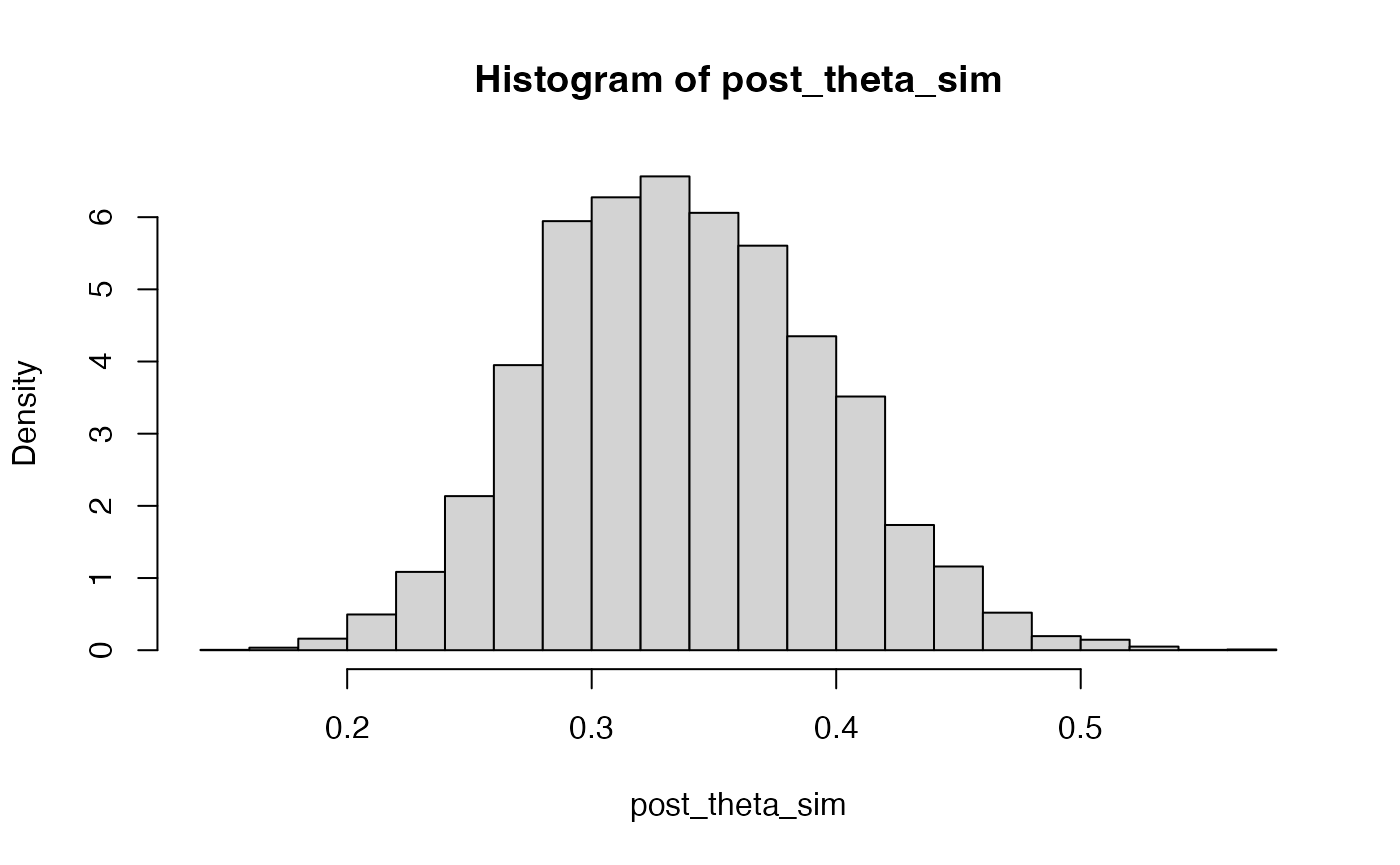

Metropolis-Hastings

As stated above, the implementation of the M-H algorithm requires a proposal distribution to obtain new values of the parameter $\theta$ . Usually, the proposal distribution is defined so that the proposed movement depends on the current value. However, in this case the proposal distribution is a log-Normal distribution centred at the logarithm of the current value with precision $100$ .

First of all, we will define the proposal distribution, prior and likelihood of the model:

# Proposal distribution: sampling
rq <- function(lambda) {
  rlnorm(1, meanlog = log(lambda), sdlog = sqrt(1 / 100))
}

# Proposal distribution: log-density
logdq <- function(new.lambda, lambda) {
  dlnorm(new.lambda, meanlog = log(lambda), sdlog = sqrt(1 / 100), log = TRUE)
}

# Prior distribution: Ga(0.01, 0.01)
logprior <- function(lambda) {
  dgamma(lambda, 0.01, 0.01, log = TRUE)
}

# LogLikelihood
loglik <- function(y, lambda) {
   res <- sum(dpois(y, lambda, log = TRUE)) 
}

Note that all densities and the likelihood are computed on the log-scale.

Next, an implementation of the M-H algorithm is as follows:

# Number of iterations
n.iter <- 40500

# Simulations of the parameter
lambda <- rep(NA, n.iter)

# Initial value
lambda[1] <- 30

for(i in 2:n.iter) {
  new.lambda <- rq(lambda[i - 1])
  
  # Log-Acceptance probability
  logacc.prob <- loglik(y, new.lambda) + logprior(new.lambda) +
    logdq(lambda[i - 1], new.lambda)
  logacc.prob <- logacc.prob - loglik(y, lambda[i - 1]) - logprior(lambda[i - 1]) - 
    logdq(new.lambda, lambda[i - 1])
  logacc.prob <- min(0, logacc.prob)#0 = log(1)
  
  if(log(runif(1)) < logacc.prob) {
    # Accept
    lambda[i] <- new.lambda
  } else {
    # Reject
    lambda[i] <- lambda[i - 1]
  }
}

The simulations we have generated are not independent of one another; each is dependent on the previous one. This has two consequences: the chain is dependent on the initial, starting value of the parameter(s); and the sampling chain itself will exhibit autocorrelation.

For this reason, we will remove the first 500 iterations to reduce the dependence of the sampling on the starting value; and we will keep only every 10^th simulation to reduce the autocorrelation in the sampled series. The 500 iterations we discard are known as the burn-in sample, and the process of keeping only every 10^th value is called thinning.

After that, we will compute summary statistics and display a density of the simulations.

# Remove burn-in
lambda <- lambda[-c(1:500)]

# Thinning
lambda <- lambda[seq(1, length(lambda), by = 10)]

# Summary statistics
summary(lambda)

##    Min. 1st Qu.  Median    Mean 3rd Qu.    Max. 
##   22.55   25.05   25.70   25.73   26.40   29.65

par(mfrow = c(1, 2))
plot(lambda, type = "l", main = "MCMC samples", ylab = expression(lambda))
plot(density(lambda), main = "Posterior density", xlab = expression(lambda))

Exercises

Performance of the proposal distribution

The proposal distribution plays a crucial role in IS and it should be as close to the posterior as possible. As a way of measuring how good a proposal distribution is, it is possible to compute the effective sample size as follows:

$\text{ESS} = \frac{(\sum_{m=1}^M w(\theta^{(m)}))^2}{\sum_{m=1}^M w(\theta^{(m)})^2}.$

Compute the effective sample size for the previous example. How is this related to the number of IS samples (n_simulations)?
Solution
```
ESS <- function(ww){
  (sum(ww)^2)/sum(ww^2)
}
ESS(ww)
```
```
## [1] 941.928
```
```
n_simulations
```
```
## [1] 10000
```

Changing the proposal distribution - Importance Sampling

Use a different proposal distribution and check how sampling weights, ESS and point estimates differ from those in the current example when using Importance Sampling. For example, a $\text{Ga}(5,\, 0.1)$ will put a higher mass on values around 40, unlike the actual posterior distribution. What differences do you find with the example presented here using a uniform proposal distribution? Why do you think that these differences appear?

Solution

n_simulations <- 10000
set.seed(12)
lambda_sim <- rgamma(n_simulations,5,0.1)
loglik_pois <- sapply(lambda_sim, function(LAMBDA) {
  sum(dpois(GoTdata$Us, LAMBDA, log = TRUE))
})
log_ww <- loglik_pois + dgamma(lambda_sim, 0.01, 0.01, log = TRUE) - dgamma(lambda_sim, 5, 0.1, log=TRUE)
log_ww <- log_ww - max(log_ww)
ww <- exp(log_ww)
ww <- ww / sum(ww)

hist(ww, xlab = "Importance weights")

post_mean <- sum(lambda_sim * ww)
post_mean

## [1] 25.70199

post_var <- sum(lambda_sim^2 * ww)- post_mean^2
post_var

## [1] 1.039709

plot(density(lambda_sim, weights = ww, bw = 0.5), main = "Posterior density", xlim = c(10,40))

ESS(ww)

## [1] 445.456

n_simulations

## [1] 10000

Changing the prior distribution - Metropolis-Hastings

We can also try using a different prior distribution on $\lambda$ , and analyse the data using the Metropolis-Hastings algorithm. Run the example for a prior distribution on $\lambda$ which is a Gamma distribution with parameters $1.0$ and $1.0$ , which is centred at 1 and has a larger precision (i.e., smaller variance) than before. How does the different prior distribution change the estimate of $\lambda$ , and why?

Solution

# Prior distribution: Ga(1.0, 1.0)
logprior <- function(lambda) {
  dgamma(lambda, 1.0, 1.0, log = TRUE)
}
# Number of iterations
n.iter <- 40500

# Simulations of the parameter
lambda <- rep(NA, n.iter)

# Initial value
lambda[1] <- 30

for(i in 2:n.iter) {
  new.lambda <- rq(lambda[i - 1])

  # Log-Acceptance probability
  logacc.prob <- loglik(y, new.lambda) + logprior(new.lambda) +
    logdq(lambda[i - 1], new.lambda)
  logacc.prob <- logacc.prob - loglik(y, lambda[i - 1]) - logprior(lambda[i - 1]) - 
    logdq(new.lambda, lambda[i - 1])
  logacc.prob <- min(0, logacc.prob)#0 = log(1)

  if(log(runif(1)) < logacc.prob) {
    # Accept
    lambda[i] <- new.lambda
  } else {
    # Reject
    lambda[i] <- lambda[i - 1]
  }
}
# Remove burn-in
lambda <- lambda[-c(1:500)]

# Thinning
lambda <- lambda[seq(1, length(lambda), by = 10)]

# Summary statistics
summary(lambda)

##    Min. 1st Qu.  Median    Mean 3rd Qu.    Max. 
##   21.69   24.12   24.76   24.77   25.42   28.48

par(mfrow = c(1, 2))
plot(lambda, type = "l", main = "MCMC samples", ylab = expression(lambda))
plot(density(lambda), main = "Posterior density", xlab = expression(lambda))

Gibbs Sampling

As we have seen in the theory session, Gibbs Sampling is an MCMC method which allows us to estimate one parameter at a time. This is very useful for models which have lots of parameters, as in a sense it reduces a very large multidimensional inference problem to a set of single dimension problems.

To recap, in order to generate a random sample from the joint density $g\left(\mathbf{\theta}\right)= g\left(\theta_1,\theta_2,\ldots,\theta_D\right)$ for a model with $D$ parameters, we use the following algorithm:

Start with an initial set $\mathbf{\theta}^{(0)}= \left(\theta_1^{(0)},\theta_2^{(0)},\ldots,\theta_D^{(0)}\right)$
Generate $\theta_1^{(1)}$ from the conditional distribution $\theta_1 \mid \left(\theta_2^{(0)},\ldots,\theta_D^{(0)}\right)$
Generate $\theta_2^{(1)}$ from the conditional distribution $\theta_2 \mid \left(\theta_1^{(1)},\theta_3^{(0)},\ldots,\theta_D^{(0)}\right)$
$\quad\quad\cdots$
Generate $\theta_D^{(1)}$ from the conditional distribution $\theta_D \mid \left(\theta_1^{(1)},\theta_2^{(1)},\ldots,\theta_{D-1}^{(1)}\right)$
Iterate from Step 2.

As with Metropolis-Hastings, in Gibbs Sampling we typically discard the initial simulations (the burn-in period), reducing the dependence on the initial set of parameter values.

As with the other MCMC algorithms, the resulting simulations approximate a random sample from the posterior distribution.

Example: Simple Linear Regression

We will illustrate the use of Gibbs Sampling on a simple linear regression model. Recall that we saw yesterday that we can obtain an analytical solution for a Bayesian linear regression, but that more complex models require a simulation approach.

The simple linear regression model we will analyse here is a reduced version of the general linear regression model we saw yesterday: $Y_i = \beta_0+\beta_1x_i+\epsilon_i$ for response variable $\mathbf{Y}=\left(Y_1,Y_2,\ldots,Y_n\right)$ , explanatory variable $\mathbf{x}=\left(x_1,x_2,\ldots,x_n\right)$ and residual vector $\mathbf{\epsilon}= \left(\epsilon_1,\epsilon_2,\ldots,\epsilon_n\right)$ for a sample of size $n$ , where $\beta_0$ is the regression intercept, $\beta_1$ is the regression slope, and where the $\epsilon_i$ are independent with $\epsilon_i\sim \textrm{N}\left(0,\sigma^2\right)$ $\forall i=1,2,\ldots,n$ . For convenience, we refer to the combined set of $\mathbf{Y}$ and $\mathbf{x}$ data as $\mathcal{D}$ . We also define $\hat{\mathbf{y}}$ to be the fitted response vector (i.e., $\hat{y}_i = \beta_0 + \beta_1 x_i$ from the regression equation) using the current values of the parameters $\beta_0$ , $\beta_1$ and precision $\tau = 1$ (remember that $\tau=\frac{1}{\sigma^2}$ ) from the Gibbs Sampling simulations.

For Bayesian inference, it is simpler to work with precisions $\tau$ rather than with variances $\sigma^2$ . Given priors $\begin{align*} \pi(\tau) &= \textrm{Ga}\left(\alpha, \beta\right), \\ \pi(\beta_0) &= \textrm{N}\left(\mu_{\beta_0}, \tau_{\beta_0}\right), \quad\textrm{and} \\ \pi(\beta_1) &= \textrm{N}\left(\mu_{\beta_1}, \tau_{\beta_1}\right). \end{align*}$ In the final Practical session later today (supplied as supplementary or advanced material) you will see this example analysed by deriving the necessary calculations needed to run the Gibbs Sampling in R without using a specific package, using the so-called “full conditional” distributions - that is, the conditional distributions referred to in the Section on Gibbs Sampling.

We will use the R package MCMCpack to run the Gibbs Sampling for this simple example, although we will use more advanced software in Practicals 6 and 7 for more complex examples.

We will study an problem from ecology, looking at the relationship between water pollution and mayfly size - the data come from the book Statistics for Ecologists Using R and Excel 2nd edition by Mark Gardener (ISBN 9781784271398), see the publisher’s webpage.

The data are as follows:

length - the length of a mayfly in mm;
BOD - biological oxygen demand in mg of oxygen per litre, effectively a measure of organic pollution (since more organic pollution requires more oxygen to break it down).

The data can be read into R:

# Read in data
BOD <- c(200,180,135,120,110,120,95,168,180,195,158,145,140,145,165,187,
         190,157,90,235,200,55,87,97,95)
mayfly.length <- c(20,21,22,23,21,20,19,16,15,14,21,21,21,20,19,18,17,19,21,13,
            16,25,24,23,22)
# Create data frame for the analysis
Data <- data.frame(BOD=BOD,mayfly.length=mayfly.length)

The package MCMCpack should be loaded into R:

library(MCMCpack)

## Loading required package: coda

## Loading required package: MASS

## ##
## ## Markov Chain Monte Carlo Package (MCMCpack)

## ## Copyright (C) 2003-2024 Andrew D. Martin, Kevin M. Quinn, and Jong Hee Park

## ##
## ## Support provided by the U.S. National Science Foundation

## ## (Grants SES-0350646 and SES-0350613)
## ##

For this Bayesian Linear Regression example, we will use the MCMCregress() function; use

?MCMCregress

to see the help page for MCMCregress(). We specify the formula just as we would for a non-Bayesian regression using the lm() function in Base R. Conjugate priors are used, with Normal priors for the regression parameters $\beta$ (with means in b0 and precisions in B0) and an inverse Gamma prior for the residual variance $\sigma^2$ ; the latter is equivalent to a Gamma prior for the residual precision $\tau$ . The parameters for the prior for $\tau$ can either be set as the shape and scale parameters of the Gamma distribution (c0/2 and d0/2 respectively) or as the mean and variance (sigma.mu and sigma.var).

Exercises

We will use Gibbs Sampling to fit a Bayesian Linear Regression model to the mayfly data. We will use the following prior distributions for the regression parameters: $\begin{align*} \pi(\tau) &= \textrm{Ga}\left(1, 1\right), \\ \pi(\beta_0) &= \textrm{N}\left(0, 0.0001\right), \quad\textrm{and} \\ \pi(\beta_1) &= \textrm{N}\left(0, 0.0001\right). \end{align*}$

We will set the initial values of both $\beta$ parameters to 1, i.e. $\beta_0^{(0)}=\beta_1^{(0)}$ . We do not need to set the initial value of $\tau$ because it is simulated first in the Gibbs Sampling within MCMCregress(). Note that MCMCregress() reports summaries of the variance $\sigma^2$ , which is helpful to us.

Data exploration

Investigate the data to see whether a linear regression model would be sensible. [Hint: a scatterplot and a correlation coefficient could be helpful.]

Solution

# Scatterplot
plot(BOD,mayfly.length)

# Correlation with hypothesis test
cor.test(BOD,mayfly.length)

## 
##  Pearson's product-moment correlation
## 
## data:  BOD and mayfly.length
## t = -6.52, df = 23, p-value = 1.185e-06
## alternative hypothesis: true correlation is not equal to 0
## 95 percent confidence interval:
##  -0.9107816 -0.6020516
## sample estimates:
##        cor 
## -0.8055507

Run a frequentist simple linear regression using the lm() function in R; this will be useful for comparison with our Bayesian analysis.

Solution

# Linear Regression using lm()
linreg <- lm(mayfly.length ~ BOD, data = Data)
summary(linreg)

## 
## Call:
## lm(formula = mayfly.length ~ BOD, data = Data)
## 
## Residuals:
##    Min     1Q Median     3Q    Max 
## -3.453 -1.073  0.307  1.105  3.343 
## 
## Coefficients:
##              Estimate Std. Error t value Pr(>|t|)    
## (Intercept) 27.697314   1.290822   21.46  < 2e-16 ***
## BOD         -0.055202   0.008467   -6.52 1.18e-06 ***
## ---
## Signif. codes:  0 '***' 0.001 '**' 0.01 '*' 0.05 '.' 0.1 ' ' 1
## 
## Residual standard error: 1.865 on 23 degrees of freedom
## Multiple R-squared:  0.6489, Adjusted R-squared:  0.6336 
## F-statistic: 42.51 on 1 and 23 DF,  p-value: 1.185e-06

Running the Gibbs Sampler

Use function MCMCregress() to fit a Bayesian simple linear regression using mayfly.length as the response variable. Ensure you have a burn-in period so that the initial simulations are discarded. You can specify the initial values of $\beta$ using the beta.start argument of MCMCregress(). The function also has the option verbose, where e.g. setting a value of 1000 implies the code will show an update to the screen every 1000 iterations.

Solution

# Bayesian Linear Regression using a Gibbs Sampler

# Set the size of the burn-in, the number of iterations of the Gibbs Sampler
# and the level of thinning
burnin <- 5000
mcmc <- 10000
thin <- 10

# Obtain the samples
results1  <- MCMCregress(mayfly.length~BOD,
                         b0=c(0.0,0.0), B0 = c(0.0001,0.0001),
                         c0 = 2, d0 = 2, # Because the prior is Ga(c0/2,d0/2),
                         beta.start = c(1,1),
                         burnin=burnin, mcmc=mcmc, thin=thin,
                         data=Data, verbose=1000)

## 
## 
## MCMCregress iteration 1 of 15000 
## beta = 
##  114.59369
##   -0.46786
## sigma2 = 21562.35575
## 
## 
## MCMCregress iteration 1001 of 15000 
## beta = 
##   28.57579
##   -0.06136
## sigma2 =    4.31350
## 
## 
## MCMCregress iteration 2001 of 15000 
## beta = 
##   24.73894
##   -0.03449
## sigma2 =    4.65105
## 
## 
## MCMCregress iteration 3001 of 15000 
## beta = 
##   28.32000
##   -0.05961
## sigma2 =    3.93605
## 
## 
## MCMCregress iteration 4001 of 15000 
## beta = 
##   26.97821
##   -0.04849
## sigma2 =    4.63895
## 
## 
## MCMCregress iteration 5001 of 15000 
## beta = 
##   27.41482
##   -0.05518
## sigma2 =    3.56662
## 
## 
## MCMCregress iteration 6001 of 15000 
## beta = 
##   31.25295
##   -0.07519
## sigma2 =    3.67459
## 
## 
## MCMCregress iteration 7001 of 15000 
## beta = 
##   28.68306
##   -0.05846
## sigma2 =    2.95033
## 
## 
## MCMCregress iteration 8001 of 15000 
## beta = 
##   28.08184
##   -0.05702
## sigma2 =    4.51031
## 
## 
## MCMCregress iteration 9001 of 15000 
## beta = 
##   26.00227
##   -0.04466
## sigma2 =    3.80170
## 
## 
## MCMCregress iteration 10001 of 15000 
## beta = 
##   27.77085
##   -0.05513
## sigma2 =    3.21633
## 
## 
## MCMCregress iteration 11001 of 15000 
## beta = 
##   29.41562
##   -0.06719
## sigma2 =    3.80747
## 
## 
## MCMCregress iteration 12001 of 15000 
## beta = 
##   29.77778
##   -0.07300
## sigma2 =    3.74206
## 
## 
## MCMCregress iteration 13001 of 15000 
## beta = 
##   26.66759
##   -0.04763
## sigma2 =    3.33029
## 
## 
## MCMCregress iteration 14001 of 15000 
## beta = 
##   29.38684
##   -0.06209
## sigma2 =    3.87291

summary(results1)

## 
## Iterations = 5001:14991
## Thinning interval = 10 
## Number of chains = 1 
## Sample size per chain = 1000 
## 
## 1. Empirical mean and standard deviation for each variable,
##    plus standard error of the mean:
## 
##                 Mean       SD  Naive SE Time-series SE
## (Intercept) 27.72514 1.346336 0.0425749      0.0425749
## BOD         -0.05551 0.008833 0.0002793      0.0002793
## sigma2       3.50903 1.049902 0.0332008      0.0301115
## 
## 2. Quantiles for each variable:
## 
##               2.5%      25%      50%      75%    97.5%
## (Intercept) 24.936 26.91014 27.76271 28.62318 30.22467
## BOD         -0.073 -0.06136 -0.05565 -0.04992 -0.03727
## sigma2       1.979  2.74378  3.37009  4.04642  6.01436

Use the function traceplot() to view the autocorrelation in the Gibbs sampling simulation chain. Is there any visual evidence of autocorrelation, or do the samples look independent?
Solution
```
par(mfrow=c(2,2))
traceplot(results1)
```
Use the function densplot() to view the shape of the posterior densities of each parameter.
Solution
```
par(mfrow=c(2,2))
densplot(results1)
```
As well as autocorrelation with single parameters, we should also be concerned about cross-correlations between different parameters - ideally these correlations would be close to zero, as parameters would be sampled at least approximately independently from each other. Use the crosscorr() function to see the cross-correlation between samples from the posterior distribution of the regression intercept and the coefficient for BOD. Are the values close to zero, or to +1 or -1?
Solution
```
crosscorr(results1)
```
```
##             (Intercept)         BOD      sigma2
## (Intercept)  1.00000000 -0.96109141 -0.05564442
## BOD         -0.96109141  1.00000000  0.04639491
## sigma2      -0.05564442  0.04639491  1.00000000
```
How do the results compare with the frequentist output?

Reducing the autocorrelation by mean-centering the covariate

One method for reducing cross-correlation between regression parameters in the sampling chains is to mean centre the covariate(s); this works because it reduces any dependence between the regression intercept and slope(s). Do this for the current example, noting that you will need to make a correction on the estimate of the regression intercept afterwards.

Solution

# Mean-centre the x covariate
DataC <- Data
meanBOD <- mean(DataC$BOD)
DataC$BOD <- DataC$BOD - meanBOD

# Set the size of the burn-in, the number of iterations of the Gibbs Sampler
# and the level of thinning
burnin <- 50000
mcmc <- 10000
thin <- 10

# Obtain the samples
results2  <- MCMCregress(mayfly.length~BOD,
                         b0=c(0.0,0.0), B0 = c(0.0001,0.0001),
                         c0 = 2, d0 = 2, # Because the prior is Ga(c0/2,d0/2),
                         beta.start = c(1,1),
                         burnin=burnin, mcmc=mcmc, thin=thin,
                         data=DataC, verbose=1000)

## 
## 
## MCMCregress iteration 1 of 60000 
## beta = 
##   34.69852
##    0.11498
## sigma2 = 2946.59852
## 
## 
## MCMCregress iteration 1001 of 60000 
## beta = 
##   19.89512
##   -0.05741
## sigma2 =    4.31326
## 
## 
## MCMCregress iteration 2001 of 60000 
## beta = 
##   18.78657
##   -0.04781
## sigma2 =    4.65200
## 
## 
## MCMCregress iteration 3001 of 60000 
## beta = 
##   19.82113
##   -0.05692
## sigma2 =    3.93707
## 
## 
## MCMCregress iteration 4001 of 60000 
## beta = 
##   19.43363
##   -0.04760
## sigma2 =    4.63958
## 
## 
## MCMCregress iteration 5001 of 60000 
## beta = 
##   19.55947
##   -0.06127
## sigma2 =    3.56661
## 
## 
## MCMCregress iteration 6001 of 60000 
## beta = 
##   20.66838
##   -0.04711
## sigma2 =    3.67427
## 
## 
## MCMCregress iteration 7001 of 60000 
## beta = 
##   19.92570
##   -0.04504
## sigma2 =    2.95035
## 
## 
## MCMCregress iteration 8001 of 60000 
## beta = 
##   19.75247
##   -0.05315
## sigma2 =    4.51008
## 
## 
## MCMCregress iteration 9001 of 60000 
## beta = 
##   19.15149
##   -0.05554
## sigma2 =    3.80059
## 
## 
## MCMCregress iteration 10001 of 60000 
## beta = 
##   19.66223
##   -0.05335
## sigma2 =    3.21754
## 
## 
## MCMCregress iteration 11001 of 60000 
## beta = 
##   20.13758
##   -0.05936
## sigma2 =    3.80684
## 
## 
## MCMCregress iteration 12001 of 60000 
## beta = 
##   20.24235
##   -0.07159
## sigma2 =    3.74353
## 
## 
## MCMCregress iteration 13001 of 60000 
## beta = 
##   19.34348
##   -0.05139
## sigma2 =    3.33079
## 
## 
## MCMCregress iteration 14001 of 60000 
## beta = 
##   20.12937
##   -0.04232
## sigma2 =    3.87363
## 
## 
## MCMCregress iteration 15001 of 60000 
## beta = 
##   19.01540
##   -0.03953
## sigma2 =    2.98221
## 
## 
## MCMCregress iteration 16001 of 60000 
## beta = 
##   19.35293
##   -0.05746
## sigma2 =    2.90274
## 
## 
## MCMCregress iteration 17001 of 60000 
## beta = 
##   19.37079
##   -0.06663
## sigma2 =    2.89264
## 
## 
## MCMCregress iteration 18001 of 60000 
## beta = 
##   19.29063
##   -0.05267
## sigma2 =    2.43528
## 
## 
## MCMCregress iteration 19001 of 60000 
## beta = 
##   19.45808
##   -0.06439
## sigma2 =    3.20901
## 
## 
## MCMCregress iteration 20001 of 60000 
## beta = 
##   19.71731
##   -0.04909
## sigma2 =    3.89850
## 
## 
## MCMCregress iteration 21001 of 60000 
## beta = 
##   19.54603
##   -0.04340
## sigma2 =    2.97958
## 
## 
## MCMCregress iteration 22001 of 60000 
## beta = 
##   19.52276
##   -0.05749
## sigma2 =    3.17695
## 
## 
## MCMCregress iteration 23001 of 60000 
## beta = 
##   19.52406
##   -0.05491
## sigma2 =    3.30296
## 
## 
## MCMCregress iteration 24001 of 60000 
## beta = 
##   19.46015
##   -0.04384
## sigma2 =    3.70693
## 
## 
## MCMCregress iteration 25001 of 60000 
## beta = 
##   19.62692
##   -0.05845
## sigma2 =    5.25006
## 
## 
## MCMCregress iteration 26001 of 60000 
## beta = 
##   19.13747
##   -0.05090
## sigma2 =    3.69566
## 
## 
## MCMCregress iteration 27001 of 60000 
## beta = 
##   19.15052
##   -0.06892
## sigma2 =    6.34844
## 
## 
## MCMCregress iteration 28001 of 60000 
## beta = 
##   19.88539
##   -0.05356
## sigma2 =    3.13399
## 
## 
## MCMCregress iteration 29001 of 60000 
## beta = 
##   18.53229
##   -0.05721
## sigma2 =    6.66909
## 
## 
## MCMCregress iteration 30001 of 60000 
## beta = 
##   19.17615
##   -0.06703
## sigma2 =    3.69534
## 
## 
## MCMCregress iteration 31001 of 60000 
## beta = 
##   19.51222
##   -0.06441
## sigma2 =    3.63189
## 
## 
## MCMCregress iteration 32001 of 60000 
## beta = 
##   20.02942
##   -0.04783
## sigma2 =    3.93347
## 
## 
## MCMCregress iteration 33001 of 60000 
## beta = 
##   19.22779
##   -0.06256
## sigma2 =    4.14724
## 
## 
## MCMCregress iteration 34001 of 60000 
## beta = 
##   19.74958
##   -0.04529
## sigma2 =    3.61764
## 
## 
## MCMCregress iteration 35001 of 60000 
## beta = 
##   19.05313
##   -0.06919
## sigma2 =    2.25023
## 
## 
## MCMCregress iteration 36001 of 60000 
## beta = 
##   20.42649
##   -0.06709
## sigma2 =    4.42822
## 
## 
## MCMCregress iteration 37001 of 60000 
## beta = 
##   20.01155
##   -0.04444
## sigma2 =    3.75874
## 
## 
## MCMCregress iteration 38001 of 60000 
## beta = 
##   19.61044
##   -0.05992
## sigma2 =    2.81824
## 
## 
## MCMCregress iteration 39001 of 60000 
## beta = 
##   20.18721
##   -0.05873
## sigma2 =    4.11590
## 
## 
## MCMCregress iteration 40001 of 60000 
## beta = 
##   19.49300
##   -0.06064
## sigma2 =    3.19911
## 
## 
## MCMCregress iteration 41001 of 60000 
## beta = 
##   18.80278
##   -0.06293
## sigma2 =    4.60514
## 
## 
## MCMCregress iteration 42001 of 60000 
## beta = 
##   19.39229
##   -0.07741
## sigma2 =    2.73323
## 
## 
## MCMCregress iteration 43001 of 60000 
## beta = 
##   19.47305
##   -0.05247
## sigma2 =    3.11187
## 
## 
## MCMCregress iteration 44001 of 60000 
## beta = 
##   20.48476
##   -0.05306
## sigma2 =    2.70580
## 
## 
## MCMCregress iteration 45001 of 60000 
## beta = 
##   19.54088
##   -0.06177
## sigma2 =    4.52469
## 
## 
## MCMCregress iteration 46001 of 60000 
## beta = 
##   19.14175
##   -0.06490
## sigma2 =    4.74373
## 
## 
## MCMCregress iteration 47001 of 60000 
## beta = 
##   19.87775
##   -0.04737
## sigma2 =    3.81238
## 
## 
## MCMCregress iteration 48001 of 60000 
## beta = 
##   20.50685
##   -0.04792
## sigma2 =    5.93746
## 
## 
## MCMCregress iteration 49001 of 60000 
## beta = 
##   19.22369
##   -0.04882
## sigma2 =    3.58456
## 
## 
## MCMCregress iteration 50001 of 60000 
## beta = 
##   19.65716
##   -0.05128
## sigma2 =    2.28963
## 
## 
## MCMCregress iteration 51001 of 60000 
## beta = 
##   18.65504
##   -0.04345
## sigma2 =    2.80696
## 
## 
## MCMCregress iteration 52001 of 60000 
## beta = 
##   19.84400
##   -0.05561
## sigma2 =    4.19969
## 
## 
## MCMCregress iteration 53001 of 60000 
## beta = 
##   19.33364
##   -0.05816
## sigma2 =    5.89947
## 
## 
## MCMCregress iteration 54001 of 60000 
## beta = 
##   20.08745
##   -0.05077
## sigma2 =    3.83621
## 
## 
## MCMCregress iteration 55001 of 60000 
## beta = 
##   20.70882
##   -0.06036
## sigma2 =    3.36468
## 
## 
## MCMCregress iteration 56001 of 60000 
## beta = 
##   19.74654
##   -0.07375
## sigma2 =    4.55154
## 
## 
## MCMCregress iteration 57001 of 60000 
## beta = 
##   19.35105
##   -0.04160
## sigma2 =    4.24165
## 
## 
## MCMCregress iteration 58001 of 60000 
## beta = 
##   20.19004
##   -0.04053
## sigma2 =    2.55143
## 
## 
## MCMCregress iteration 59001 of 60000 
## beta = 
##   19.66103
##   -0.05363
## sigma2 =    2.07754

summary(results2)

## 
## Iterations = 50001:59991
## Thinning interval = 10 
## Number of chains = 1 
## Sample size per chain = 1000 
## 
## 1. Empirical mean and standard deviation for each variable,
##    plus standard error of the mean:
## 
##                 Mean      SD  Naive SE Time-series SE
## (Intercept) 19.61403 0.37599 0.0118898      0.0100889
## BOD         -0.05478 0.00862 0.0002726      0.0002552
## sigma2       3.47803 1.07811 0.0340929      0.0340929
## 
## 2. Quantiles for each variable:
## 
##                 2.5%      25%      50%      75%    97.5%
## (Intercept) 18.84960 19.36318 19.63098 19.86544 20.34886
## BOD         -0.07067 -0.06099 -0.05491 -0.04897 -0.03778
## sigma2       2.01223  2.72506  3.27807  3.98491  6.20298

# Correct the effect of the mean-centering on the intercept, using the
# full set of simulated outputs
results2.simulations <- as.data.frame(results2)
results2.beta.0 <- results2.simulations[,"(Intercept)"] - meanBOD * results2.simulations$BOD
summary(results2.beta.0)

##    Min. 1st Qu.  Median    Mean 3rd Qu.    Max. 
##   22.78   26.77   27.64   27.61   28.49   31.96

var(results2.beta.0)

## [1] 1.704337

sd(results2.beta.0)

## [1] 1.305503

Look at the trace plots, density plots and cross-correlations as before. Are there any notable differences when mean-centering the covariate, especially with regard to the cross-correlations?

Solution

par(mfrow=c(2,2))
traceplot(results2)

par(mfrow=c(2,2))
densplot(results2)
# Need to use the Base R kernel density function to look at the corrected 
# Intercept
plot(density(results2.beta.0, bw = 0.3404), xlim=c(22,34),
     main = "Density, corrected Intercept")

crosscorr(results2)

##              (Intercept)         BOD       sigma2
## (Intercept)  1.000000000  0.02131006 -0.001004385
## BOD          0.021310056  1.00000000 -0.019271243
## sigma2      -0.001004385 -0.01927124  1.000000000

VIBASS

Introduction

Importance Sampling

The Metropolis-Hastings Algorithm

Example: Poisson-Gamma Model

Importance sampling

Metropolis-Hastings

Exercises

Performance of the proposal distribution

Changing the proposal distribution - Importance Sampling

Changing the prior distribution - Metropolis-Hastings

Gibbs Sampling

Example: Simple Linear Regression

Exercises

Data exploration

Running the Gibbs Sampler

Reducing the autocorrelation by mean-centering the covariate