Practical 7: Bayesian Hierarchical Modelling

Bayesian Hierarchical Modelling

In this last practical we will consider the analysis of Bayesian hierarchical models. As explained in the previous lecture, hierarchical models provide a convenient tool to define models so that the different sources of variation in the data are clearly identified. Bayesian inference for highly structured hierarchical models can be difficult and may require the use of Markov chain Monte Carlo methods. However, packages such as BayesX and INLA, to mention just two, provide a very convenient way to fit and make inference about certain types of Bayesian hierarchical models.

Regarding software, we will use INLA to fit the models in the examples from this point on. The reason is that it is a popular software for Bayesian inference and very fast.

Linear Mixed Models

Linear mixed models were defined in the lecture as follows:

\[ Y_{ij} = X_{ij}\beta +\phi_i+\epsilon_{ij} \]

Here, Y_{ij} represents observation \(j\) in group \(i\), X_{ij} are a vector of covariates with coefficients \(\beta\), \(\phi_i\) i.i.d. random effects and \(\epsilon_{ij}\) a Gaussian error term. The distribution of the random effects \(\phi_i\) is Gaussian with zero mean and precision \(\tau_{\phi}\).

Multilevel Modelling

Multilevel models are a particular type of mixed-effects models in which observations are nested within groups, so that group effects are modelled using random effects. A typical example is that of students nested within classes.

For the next example, the nlschools data set (in package MASS) will be used. This data set records data about students’ performance (in particular, about a language score test) and other variables. The variables in this data set are:

lang, language score test.
IQ, verbal IQ.
class, class ID.
GS, class size as number of eighth-grade pupils recorded in the class.
SES, social-economic status of pupil’s family.
COMB, whether the pupils are taught in the multi-grade class with 7th-grade students.

The data set can be loaded and summarised as follows:

library("MASS")
data("nlschools")
summary(nlschools)

##       lang             IQ            class            GS             SES       
##  Min.   : 9.00   Min.   : 4.00   15580  :  33   Min.   :10.00   Min.   :10.00  
##  1st Qu.:35.00   1st Qu.:10.50   5480   :  31   1st Qu.:23.00   1st Qu.:20.00  
##  Median :42.00   Median :12.00   15980  :  31   Median :27.00   Median :27.00  
##  Mean   :40.93   Mean   :11.83   16180  :  31   Mean   :26.51   Mean   :27.81  
##  3rd Qu.:48.00   3rd Qu.:13.00   18380  :  31   3rd Qu.:31.00   3rd Qu.:35.00  
##  Max.   :58.00   Max.   :18.00   5580   :  30   Max.   :39.00   Max.   :50.00  
##                                  (Other):2100                                  
##  COMB    
##  0:1658  
##  1: 629  
##          
##          
##          
##          
##

The model to fit will take lang as the response variable and include IQ, GS, SES and COMB as covariates (i.e., fixed effects). This model can easily be fit with INLA as follows:

library("INLA")
m1 <- inla(lang ~ IQ + GS +  SES + COMB, data = nlschools)

summary(m1)

## 
## Call:
##    c("inla.core(formula = formula, family = family, contrasts = contrasts, 
##    ", " data = data, quantiles = quantiles, E = E, offset = offset, ", " 
##    scale = scale, weights = weights, Ntrials = Ntrials, strata = strata, 
##    ", " lp.scale = lp.scale, link.covariates = link.covariates, verbose = 
##    verbose, ", " lincomb = lincomb, selection = selection, control.compute 
##    = control.compute, ", " control.predictor = control.predictor, 
##    control.family = control.family, ", " control.inla = control.inla, 
##    control.fixed = control.fixed, ", " control.mode = control.mode, 
##    control.expert = control.expert, ", " control.hazard = control.hazard, 
##    control.lincomb = control.lincomb, ", " control.update = 
##    control.update, control.lp.scale = control.lp.scale, ", " 
##    control.pardiso = control.pardiso, only.hyperparam = only.hyperparam, 
##    ", " inla.call = inla.call, inla.arg = inla.arg, num.threads = 
##    num.threads, ", " blas.num.threads = blas.num.threads, keep = keep, 
##    working.directory = working.directory, ", " silent = silent, inla.mode 
##    = inla.mode, safe = FALSE, debug = debug, ", " .parent.frame = 
##    .parent.frame)") 
## Time used:
##     Pre = 4.41, Running = 1.09, Post = 0.0403, Total = 5.54 
## Fixed effects:
##               mean    sd 0.025quant 0.5quant 0.975quant   mode kld
## (Intercept)  9.685 1.070      7.586    9.685     11.784  9.685   0
## IQ           2.391 0.074      2.246    2.391      2.536  2.391   0
## GS          -0.026 0.025     -0.076   -0.026      0.024 -0.026   0
## SES          0.148 0.014      0.120    0.148      0.175  0.148   0
## COMB1       -1.684 0.325     -2.322   -1.684     -1.047 -1.684   0
## 
## Model hyperparameters:
##                                          mean    sd 0.025quant 0.5quant
## Precision for the Gaussian observations 0.021 0.001       0.02    0.021
##                                         0.975quant  mode
## Precision for the Gaussian observations      0.022 0.021
## 
## Marginal log-Likelihood:  -7713.46 
##  is computed 
## Posterior summaries for the linear predictor and the fitted values are computed
## (Posterior marginals needs also 'control.compute=list(return.marginals.predictor=TRUE)')

Note that the previous model only includes fixed effects. The data set includes class as the class ID to which each student belongs. Class effects can have an impact on the performance of the students, with students in the same class performing similarly in the language test.

Very conveniently, INLA can include random effects in the model by adding a term in the right hand side of the formula that defined the model. Specifically, the term to add is f(class, model = "iid") (see code below for the full model). This will create a random effect indexed over variable class and which is of type iid, i.e., the random effects are independent and identically distributed using a normal distribution with zero mean and precision \(\tau\).

Before fitting the model, the between-class variability can be explored by means of boxplots:

boxplot(lang ~ class, data = nlschools, las = 2)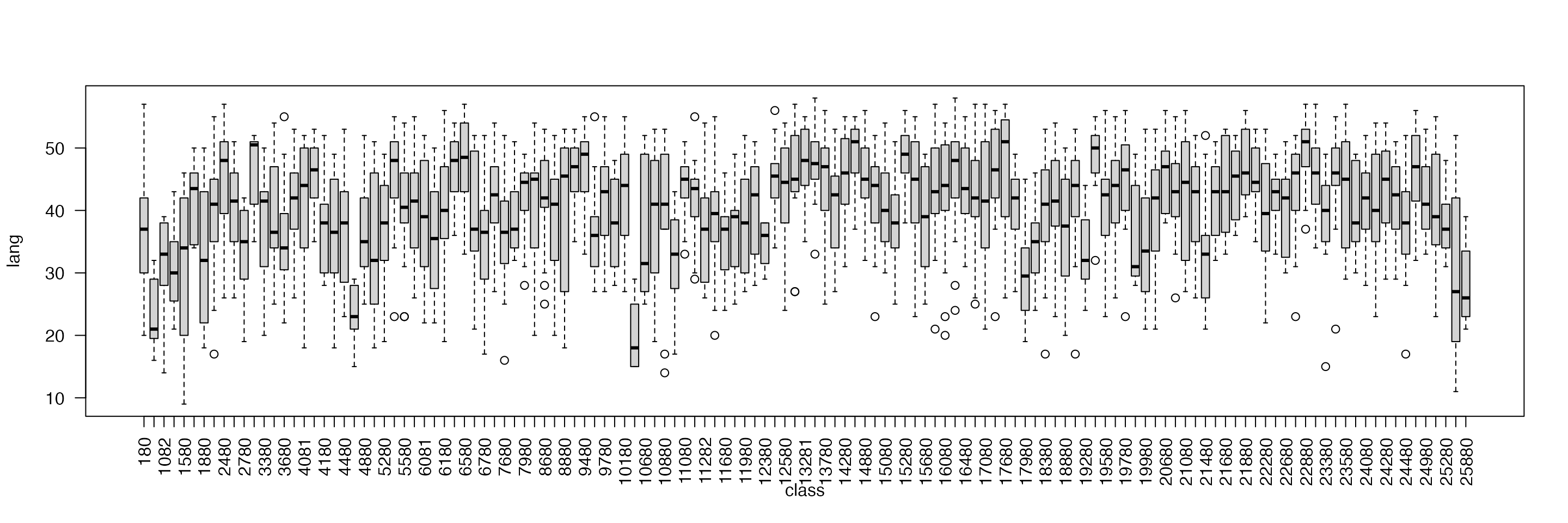

The code to fit the model with random effects is:

m2 <- inla(
  lang ~ IQ + GS +  SES + COMB + f(class, model = "iid"),
  data = nlschools
)

## 
##  *** inla.core.safe:  rerun to try to solve negative eigenvalue(s) in the Hessian

summary(m2)

## 
## Call:
##    c("inla.core(formula = formula, family = family, contrasts = contrasts, 
##    ", " data = data, quantiles = quantiles, E = E, offset = offset, ", " 
##    scale = scale, weights = weights, Ntrials = Ntrials, strata = strata, 
##    ", " lp.scale = lp.scale, link.covariates = link.covariates, verbose = 
##    verbose, ", " lincomb = lincomb, selection = selection, control.compute 
##    = control.compute, ", " control.predictor = control.predictor, 
##    control.family = control.family, ", " control.inla = control.inla, 
##    control.fixed = control.fixed, ", " control.mode = control.mode, 
##    control.expert = control.expert, ", " control.hazard = control.hazard, 
##    control.lincomb = control.lincomb, ", " control.update = 
##    control.update, control.lp.scale = control.lp.scale, ", " 
##    control.pardiso = control.pardiso, only.hyperparam = only.hyperparam, 
##    ", " inla.call = inla.call, inla.arg = inla.arg, num.threads = 
##    num.threads, ", " blas.num.threads = blas.num.threads, keep = keep, 
##    working.directory = working.directory, ", " silent = silent, inla.mode 
##    = inla.mode, safe = FALSE, debug = debug, ", " .parent.frame = 
##    .parent.frame)") 
## Time used:
##     Pre = 2.26, Running = 0.894, Post = 0.037, Total = 3.19 
## Fixed effects:
##               mean    sd 0.025quant 0.5quant 0.975quant   mode kld
## (Intercept)  9.685 1.071      7.585    9.685     11.785  9.685   0
## IQ           2.391 0.074      2.245    2.391      2.536  2.391   0
## GS          -0.026 0.025     -0.076   -0.026      0.024 -0.026   0
## SES          0.148 0.014      0.120    0.148      0.175  0.148   0
## COMB1       -1.684 0.325     -2.322   -1.684     -1.046 -1.684   0
## 
## Random effects:
##   Name     Model
##     class IID model
## 
## Model hyperparameters:
##                                             mean       sd 0.025quant 0.5quant
## Precision for the Gaussian observations 2.10e-02 1.00e-03       0.02  2.1e-02
## Precision for class                     1.99e+04 1.97e+04    1300.43  1.4e+04
##                                         0.975quant     mode
## Precision for the Gaussian observations   2.20e-02    0.021
## Precision for class                       7.22e+04 3527.201
## 
## Marginal log-Likelihood:  -7713.67 
##  is computed 
## Posterior summaries for the linear predictor and the fitted values are computed
## (Posterior marginals needs also 'control.compute=list(return.marginals.predictor=TRUE)')

Generalised Linear Mixed Models

Mixed effects models can also be considered within the context of generalised linear models. In this case, the linear predictor of observation \(i\), \(\eta_i\), can be defined as

\[ \eta_i = X_{ij}\beta +\phi_i \]

Compared to the previous setting of linear mixed effects models, note that now the distribution of the response could be other than Gaussian and that observations are not necessarily nested within groups.

Poisson regression

In this practical we will use the North Carolina Sudden Infant Death Syndrome (SIDS) data set. It is available in the spData package and it can be loaded using:

library(spData)
data(nc.sids)
summary(nc.sids)

##     CNTY.ID         BIR74           SID74          NWBIR74      
##  Min.   :1825   Min.   :  248   Min.   : 0.00   Min.   :   1.0  
##  1st Qu.:1902   1st Qu.: 1077   1st Qu.: 2.00   1st Qu.: 190.0  
##  Median :1982   Median : 2180   Median : 4.00   Median : 697.5  
##  Mean   :1986   Mean   : 3300   Mean   : 6.67   Mean   :1051.0  
##  3rd Qu.:2067   3rd Qu.: 3936   3rd Qu.: 8.25   3rd Qu.:1168.5  
##  Max.   :2241   Max.   :21588   Max.   :44.00   Max.   :8027.0  
##      BIR79           SID79          NWBIR79             east      
##  Min.   :  319   Min.   : 0.00   Min.   :    3.0   Min.   : 19.0  
##  1st Qu.: 1336   1st Qu.: 2.00   1st Qu.:  250.5   1st Qu.:178.8  
##  Median : 2636   Median : 5.00   Median :  874.5   Median :285.0  
##  Mean   : 4224   Mean   : 8.36   Mean   : 1352.8   Mean   :271.3  
##  3rd Qu.: 4889   3rd Qu.:10.25   3rd Qu.: 1406.8   3rd Qu.:361.2  
##  Max.   :30757   Max.   :57.00   Max.   :11631.0   Max.   :482.0  
##      north             x                 y             lon        
##  Min.   :  6.0   Min.   :-328.04   Min.   :3757   Min.   :-84.08  
##  1st Qu.: 97.0   1st Qu.: -60.55   1st Qu.:3920   1st Qu.:-81.20  
##  Median :125.5   Median : 114.38   Median :3963   Median :-79.26  
##  Mean   :122.1   Mean   :  91.46   Mean   :3953   Mean   :-79.51  
##  3rd Qu.:151.5   3rd Qu.: 240.03   3rd Qu.:4000   3rd Qu.:-77.87  
##  Max.   :182.0   Max.   : 439.65   Max.   :4060   Max.   :-75.67  
##       lat             L.id           M.id     
##  Min.   :33.92   Min.   :1.00   Min.   :1.00  
##  1st Qu.:35.26   1st Qu.:1.00   1st Qu.:2.00  
##  Median :35.68   Median :2.00   Median :3.00  
##  Mean   :35.62   Mean   :2.12   Mean   :2.67  
##  3rd Qu.:36.05   3rd Qu.:3.00   3rd Qu.:3.25  
##  Max.   :36.52   Max.   :4.00   Max.   :4.00

A full description of the data set is provided in the associated manual page (check with ?nc.sids) but in this practical we will only consider these variables:

BIR74, number of births (1974-78).
SID74, number of SID deaths (1974-78).
NWBIR74, number of non-white births (1974-78).

These variables are measured at the county level in North Carolina, of which there are 100.

Because SID74 records the number of SID deaths, the model is Poisson:

\[ O_i \mid \mu_i \sim Po(\mu_i),\ i=1,\ldots, 100 \] Here, \(O_i\) represents the number of cases in county \(i\) and \(\mu_i\) the mean. In addition, mean \(\mu_i\) will be written as \(\mu_i = E_i \theta_i\), where \(E_i\) is the expected number of cases and \(\theta_i\) the relative risk in county \(i\).

The relative risk \(\theta_i\) is often modelled, on the log-scale, to be equal to a linear predictor:

\[ \log(\theta_i) = \beta_0 + \ldots \]

The expected number of cases is computed by multiplying the number of births in county \(i\) to the overall mortality rate

\[ r = \frac{\sum_{i=1}^{100}O_i}{\sum_{i=1}^{100}B_i} \] where \(B_i\) represents the total number of births in country \(i\). Hence, the expected number of cases in county \(i\) is \(E_i = r B_i\).

# Overall mortality rate
r74 <- sum(nc.sids$SID74) / sum(nc.sids$BIR74)
# Expected cases
nc.sids$EXP74 <- r74 * nc.sids$BIR74

A common measure of relative risk is the standardised mortality ratio (\(O_i / E_i\)):

nc.sids$SMR74 <- nc.sids$SID74 / nc.sids$EXP74

A summary of the SMR can be obtained:

hist(nc.sids$SMR, xlab = "SMR")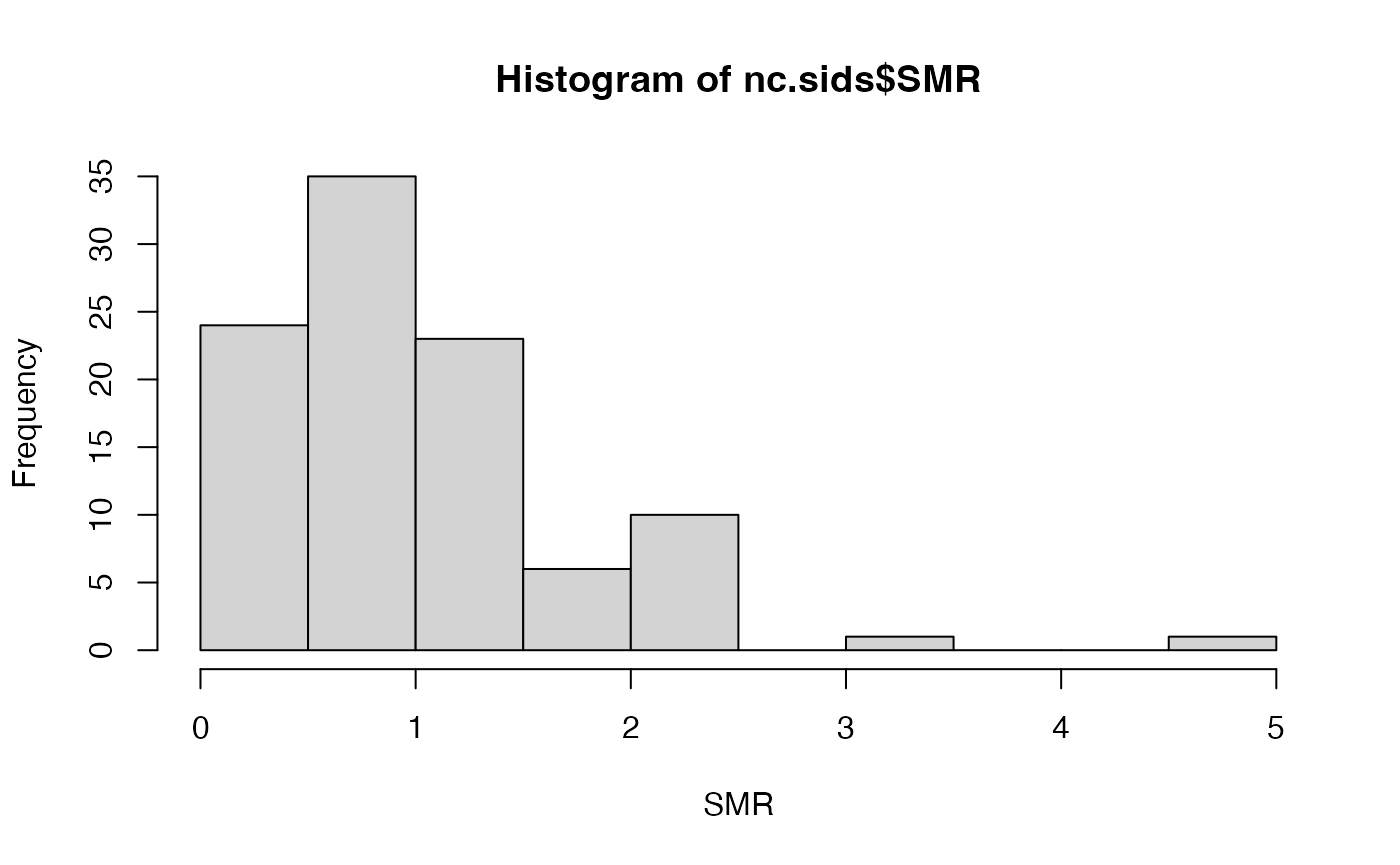

Values above 1 indicate that the county has more observed deaths than expected and that there might be an increased risk in the area.

As a covariate, we will compute the proportion of non-white births:

nc.sids$NWPROP74 <- nc.sids$NWBIR74/ nc.sids$BIR74

There is a clear relationship between the SMR and the proportion of non-white births in a county:

plot(nc.sids$NWPROP74, nc.sids$SMR74)

# Correlation
cor(nc.sids$NWPROP74, nc.sids$SMR74)

## [1] 0.5793901

A simple Poisson regression can be fit by using the following code:

m1nc <- inla(
  SID74 ~ 1 + NWPROP74,
  family = "poisson",
  E = nc.sids$EXP74,
  data = nc.sids
)
summary(m1nc)

## 
## Call:
##    c("inla.core(formula = formula, family = family, contrasts = contrasts, 
##    ", " data = data, quantiles = quantiles, E = E, offset = offset, ", " 
##    scale = scale, weights = weights, Ntrials = Ntrials, strata = strata, 
##    ", " lp.scale = lp.scale, link.covariates = link.covariates, verbose = 
##    verbose, ", " lincomb = lincomb, selection = selection, control.compute 
##    = control.compute, ", " control.predictor = control.predictor, 
##    control.family = control.family, ", " control.inla = control.inla, 
##    control.fixed = control.fixed, ", " control.mode = control.mode, 
##    control.expert = control.expert, ", " control.hazard = control.hazard, 
##    control.lincomb = control.lincomb, ", " control.update = 
##    control.update, control.lp.scale = control.lp.scale, ", " 
##    control.pardiso = control.pardiso, only.hyperparam = only.hyperparam, 
##    ", " inla.call = inla.call, inla.arg = inla.arg, num.threads = 
##    num.threads, ", " blas.num.threads = blas.num.threads, keep = keep, 
##    working.directory = working.directory, ", " silent = silent, inla.mode 
##    = inla.mode, safe = FALSE, debug = debug, ", " .parent.frame = 
##    .parent.frame)") 
## Time used:
##     Pre = 3.35, Running = 0.45, Post = 0.0136, Total = 3.81 
## Fixed effects:
##               mean    sd 0.025quant 0.5quant 0.975quant   mode kld
## (Intercept) -0.647 0.090     -0.824   -0.647     -0.471 -0.647   0
## NWPROP74     1.867 0.217      1.441    1.867      2.293  1.867   0
## 
## Marginal log-Likelihood:  -226.13 
##  is computed 
## Posterior summaries for the linear predictor and the fitted values are computed
## (Posterior marginals needs also 'control.compute=list(return.marginals.predictor=TRUE)')

Random effects can also be included to account for intrinsic differences between the counties:

# Index for random effects
nc.sids$ID <- 1:nrow(nc.sids)

# Model WITH covariate
m2nc <- inla(
  SID74 ~  1 + NWPROP74 + f(ID, model = "iid"),
  family = "poisson",
  E = nc.sids$EXP74,
  data = as.data.frame(nc.sids)
)

summary(m2nc)

## 
## Call:
##    c("inla.core(formula = formula, family = family, contrasts = contrasts, 
##    ", " data = data, quantiles = quantiles, E = E, offset = offset, ", " 
##    scale = scale, weights = weights, Ntrials = Ntrials, strata = strata, 
##    ", " lp.scale = lp.scale, link.covariates = link.covariates, verbose = 
##    verbose, ", " lincomb = lincomb, selection = selection, control.compute 
##    = control.compute, ", " control.predictor = control.predictor, 
##    control.family = control.family, ", " control.inla = control.inla, 
##    control.fixed = control.fixed, ", " control.mode = control.mode, 
##    control.expert = control.expert, ", " control.hazard = control.hazard, 
##    control.lincomb = control.lincomb, ", " control.update = 
##    control.update, control.lp.scale = control.lp.scale, ", " 
##    control.pardiso = control.pardiso, only.hyperparam = only.hyperparam, 
##    ", " inla.call = inla.call, inla.arg = inla.arg, num.threads = 
##    num.threads, ", " blas.num.threads = blas.num.threads, keep = keep, 
##    working.directory = working.directory, ", " silent = silent, inla.mode 
##    = inla.mode, safe = FALSE, debug = debug, ", " .parent.frame = 
##    .parent.frame)") 
## Time used:
##     Pre = 4.29, Running = 0.752, Post = 0.0244, Total = 5.07 
## Fixed effects:
##               mean    sd 0.025quant 0.5quant 0.975quant   mode kld
## (Intercept) -0.650 0.104     -0.856   -0.650     -0.447 -0.649   0
## NWPROP74     1.883 0.253      1.387    1.882      2.384  1.880   0
## 
## Random effects:
##   Name     Model
##     ID IID model
## 
## Model hyperparameters:
##                    mean     sd 0.025quant 0.5quant 0.975quant  mode
## Precision for ID 134.13 229.40       9.57    31.05     416.29 15.76
## 
## Marginal log-Likelihood:  -227.83 
##  is computed 
## Posterior summaries for the linear predictor and the fitted values are computed
## (Posterior marginals needs also 'control.compute=list(return.marginals.predictor=TRUE)')

The role of the covariate can be explored by fitting a model without it:

# Model WITHOUT covariate
m3nc <- inla(
  SID74 ~  1 + f(ID, model = "iid"),
  family = "poisson",
  E = nc.sids$EXP74,
  data = as.data.frame(nc.sids)
)

summary(m3nc)

## 
## Call:
##    c("inla.core(formula = formula, family = family, contrasts = contrasts, 
##    ", " data = data, quantiles = quantiles, E = E, offset = offset, ", " 
##    scale = scale, weights = weights, Ntrials = Ntrials, strata = strata, 
##    ", " lp.scale = lp.scale, link.covariates = link.covariates, verbose = 
##    verbose, ", " lincomb = lincomb, selection = selection, control.compute 
##    = control.compute, ", " control.predictor = control.predictor, 
##    control.family = control.family, ", " control.inla = control.inla, 
##    control.fixed = control.fixed, ", " control.mode = control.mode, 
##    control.expert = control.expert, ", " control.hazard = control.hazard, 
##    control.lincomb = control.lincomb, ", " control.update = 
##    control.update, control.lp.scale = control.lp.scale, ", " 
##    control.pardiso = control.pardiso, only.hyperparam = only.hyperparam, 
##    ", " inla.call = inla.call, inla.arg = inla.arg, num.threads = 
##    num.threads, ", " blas.num.threads = blas.num.threads, keep = keep, 
##    working.directory = working.directory, ", " silent = silent, inla.mode 
##    = inla.mode, safe = FALSE, debug = debug, ", " .parent.frame = 
##    .parent.frame)") 
## Time used:
##     Pre = 4.83, Running = 0.949, Post = 0.0283, Total = 5.8 
## Fixed effects:
##              mean    sd 0.025quant 0.5quant 0.975quant   mode kld
## (Intercept) -0.03 0.063     -0.157   -0.028      0.091 -0.026   0
## 
## Random effects:
##   Name     Model
##     ID IID model
## 
## Model hyperparameters:
##                  mean   sd 0.025quant 0.5quant 0.975quant mode
## Precision for ID 7.26 2.57       3.79     6.77      13.56 6.00
## 
## Marginal log-Likelihood:  -245.56 
##  is computed 
## Posterior summaries for the linear predictor and the fitted values are computed
## (Posterior marginals needs also 'control.compute=list(return.marginals.predictor=TRUE)')

Now, notice the decrease in the estimate of the precision of the random effects (i.e., the variance increases). This means that values of the random effects are now larger than in the previous case as the random effects pick some of the effect explained by the covariate.

par(mfrow = c(1, 2))
boxplot(m2nc$summary.random$ID$mean, ylim = c(-1, 1), main = "With NWPROP74")
boxplot(m3nc$summary.random$ID$mean, ylim = c(-1, 1), main = "Without NWPROP74")

Further Extensions

Spatial random effects can be defined not to be independent and identically distributed. Instead, spatial or temporal correlation can be considered when defining them. For example, in the North Carolina SIDS data set, it is common to consider that two counties that are neighbours (i.e., share a boundary) will have similar relative risks. This can be taken into account in the model but assuming that the random effects are spatially autocorrelated. This is out of the scope of this introductory course but feel free to ask about this!!

VIBASS

Bayesian Hierarchical Modelling

Linear Mixed Models

Multilevel Modelling

Generalised Linear Mixed Models

Poisson regression

Further Extensions