Introduction
This practical is entirely optional, and presents additional and advanced material you may wish to try out if you have completed all the work in the first seven practicals, and have no further questions for us.
We start with an example where we implement specific R code for
running the linear regression example of Practical 5; then we repeat the
examples of Practicals 6 and 7 but using INLA rather than
BayesX. Note we did not include INLA examples
in the main material as we did not want to have too many different
packages included, which would detract from the most important part -
learning about Bayesian Statistics!
Example: Simple Linear Regression
We will illustrate the use of Gibbs Sampling on a simple linear
regression model. Recall that we saw yesterday that we can obtain an
analytical solution for a Bayesian linear regression, but that more
complex models require a simulation approach; in Practical 5, we used
the package MCMCpack to fit the model using Gibbs
Sampling.
The approach we take here for Gibbs Sampling on a simple linear regression model is very easily generalised to more complex models, the key is that whatever your model looks like, you update one parameter at a time, using the conditional distribution of that parameter given the current values of all the other parameters.
The simple linear regression model we will analyse here is a reduced version of the general linear regression model we saw yesterday, and the same one as in Practical 5: for response variable , explanatory variable and residual vector for a sample of size , where is the regression intercept, is the regression slope, and where the are independent with . For convenience, we refer to the combined set of and data as . We also define to be the fitted response vector (i.e., from the regression equation) using the current values of the parameters , and precision (remember that ) from the Gibbs Sampling simulations.
For Bayesian inference, it is simpler to work with precisions rather than with variances . Given priors then by combining with the likelihood we can derive the full conditional distributions for each parameter. For , we have For we will need to expand , and then we have
In the above, represents a quantity that is constant with respect to and hence can be ignored. Finally, for we have This gives us an easy way to run Gibbs Sampling for linear regression; we have standard distributions as full conditionals and there are standard functions in R to obtain the simulations.
We shall do this now for an example in ecology, looking at the relationship between water pollution and mayfly size - the data come from the book Statistics for Ecologists Using R and Excel 2nd edition by Mark Gardener (ISBN 9781784271398), see the publisher’s webpage.
The data are as follows:
length- the length of a mayfly in mm;BOD- biological oxygen demand in mg of oxygen per litre, effectively a measure of organic pollution (since more organic pollution requires more oxygen to break it down).
The data can be read into R:
# Read in data
BOD <- c(200,180,135,120,110,120,95,168,180,195,158,145,140,145,165,187,
         190,157,90,235,200,55,87,97,95)
mayfly.length <- c(20,21,22,23,21,20,19,16,15,14,21,21,21,20,19,18,17,19,21,13,
            16,25,24,23,22)
# Create data frame for the Gibbs Sampling, needs x and y
Data <- data.frame(x=BOD,y=mayfly.length)
We provide here some simple functions for running the analysis by
Gibbs Sampling, using the full conditionals derived above. The functions
assume you have a data frame with two columns, the response
y and the covariate x.
# Function to update tau, the precision
sample_tau <- function(data, beta0, beta1, alphatau, betatau) {
  rgamma(1,
    shape = alphatau+ nrow(data) / 2,
    rate = betatau+ 0.5 * sum((data$y - (beta0 + data$x*beta1))^2)
  )
}

# Function to update beta0, the regression intercept
sample_beta0 <- function(data, beta1, tau, mu0, tau0) {
  prec <- tau0 + tau * nrow(data)
  mean <- (tau0*mu0 + tau * sum(data$y - data$x*beta1)) / prec
  rnorm(1, mean = mean, sd = 1 / sqrt(prec))
}

# Function to update beta1, the regression slope
sample_beta1 <- function(data, beta0, tau, mu1, tau1) {
  prec <- tau1 + tau * sum(data$x * data$x)
  mean <- (tau1*mu1 + tau * sum((data$y - beta0) * data$x)) / prec
  rnorm(1, mean = mean, sd = 1 / sqrt(prec))
}

# Function to run the Gibbs Sampling, where you specify the number of
# simulations `m`, the starting values for each of the three regression
# parameters (`tau_start` etc), and the parameters for the prior
# distributions of tau, beta0 and beta1
gibbs_sample <- function(data,
                         tau_start,
                         beta0_start,
                         beta1_start,
                         m,
                         alpha_tau,
                         beta_tau,
                         mu_beta0,
                         tau_beta0,
                         mu_beta1,
                         tau_beta1) {
  tau <- numeric(m)
  beta0 <- numeric(m)
  beta1 <- numeric(m)
  tau[1] <- tau_start
  beta0[1] <- beta0_start
  beta1[1] <- beta1_start

  for (i in 2:m) {
    tau[i] <-
      sample_tau(data, beta0[i-1], beta1[i-1], alpha_tau, beta_tau)
    beta0[i] <-
      sample_beta0(data, beta1[i-1], tau[i], mu_beta0, tau_beta0)
    beta1[i] <-
    sample_beta1(data, beta0[i], tau[i], mu_beta1, tau_beta1)
  }

  Iteration <- 1:m
  data.frame(Iteration,beta0,beta1,tau)
}
Exercises
We will use Gibbs Sampling to fit a Bayesian Linear Regression model to the mayfly data, with the above code. We will use the following prior distributions for the regression parameters: We will set the initial values of all parameters to 1, i.e. .
Data exploration
-
Investigate the data to see whether a linear regression model would be sensible. [You may not need to do this step if you recall the outputs from Practical 5.]
Solution
# Scatterplot plot(BOD,mayfly.length)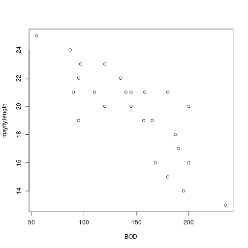 plot of chunk unnamed-chunk-3
# Correlation with hypothesis test
cor.test(BOD,mayfly.length)
## ## Pearson's product-moment correlation ## ## data: BOD and mayfly.length ## t = -6.52, df = 23, p-value = 1.185e-06 ## alternative hypothesis: true correlation is not equal to 0 ## 95 percent confidence interval: ## -0.9107816 -0.6020516 ## sample estimates: ## cor ## -0.8055507 -
Run a frequentist simple linear regression using the
lmfunction in R; this will be useful for comparison with our Bayesian analysis.Solution
##
## Call:
## lm(formula = mayfly.length ~ BOD, data = Data)
##
## Residuals:
##    Min     1Q Median     3Q    Max
## -3.453 -1.073  0.307  1.105  3.343
##
## Coefficients:
##              Estimate Std. Error t value Pr(>|t|)
## (Intercept) 27.697314   1.290822   21.46  < 2e-16 ***
## BOD         -0.055202   0.008467   -6.52 1.18e-06 ***
## ---
## Signif. codes:  0 '***' 0.001 '**' 0.01 '*' 0.05 '.' 0.1 ' ' 1
##
## Residual standard error: 1.865 on 23 degrees of freedom
## Multiple R-squared:  0.6489, Adjusted R-squared:  0.6336
## F-statistic: 42.51 on 1 and 23 DF,  p-value: 1.185e-06
Running the Gibbs Sampler
-
Use the code above to fit a Bayesian simple linear regression using
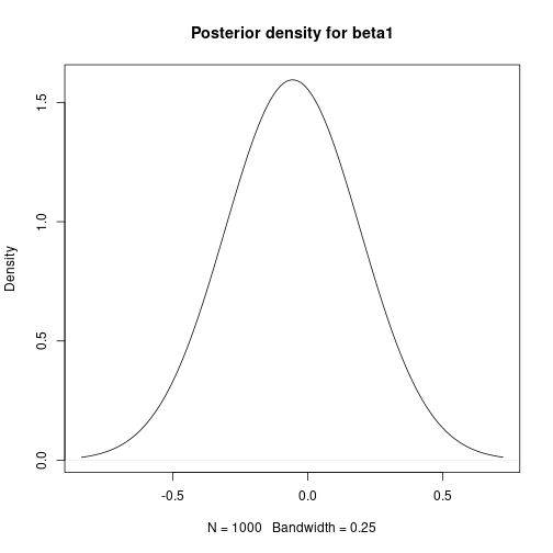
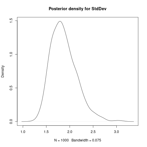
lengthas the response variable. Ensure you have a burn-in period so that the initial simulations are discarded. Use the output fromgibbs_sampleto estimate the regression parameters (with uncertainty measures). Also plot the estimates of the posterior distributions.Solution
# Bayesian Linear Regression using a Gibbs Sampler

# Set the number of iterations of the Gibbs Sampler - including how many to
# discard as the burn-in
m.burnin <- 500
m.keep <- 1000
m <- m.burnin + m.keep

# Obtain the samples
results1 <- gibbs_sample(Data,1,1,1,m,1,1,0,0.0001,0,0.0001)
# Remove the burn-in
results1 <- results1[-(1:m.burnin),]
# Add variance and standard deviation columns
results1$Variance <- 1/results1$tau
results1$StdDev <- sqrt(results1$Variance)
# Estimates are the column means
apply(results1[,-1],2,mean)
## beta0 beta1 tau Variance StdDev ## 27.65318069 -0.05486106 0.30030561 3.64651228 1.88708959# Also look at uncertainty apply(results1[,-1],2,sd)## beta0 beta1 tau Variance StdDev ## 1.333977050 0.008754095 0.088994547 1.180979250 0.292387827## beta0 beta1 tau Variance StdDev ## 2.5% 24.94863 -0.07188798 0.1532262 1.997486 1.413324 ## 97.5% 30.31030 -0.03701739 0.5006294 6.526298 2.554662# Kernel density plots for beta0, beta1 and the residual stanard deviation plot(density(results1$beta0, bw = 0.5), main = "Posterior density for beta0")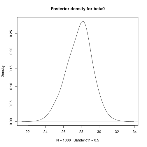 plot of chunk unnamed-chunk-5
 plot of chunk unnamed-chunk-5
 plot of chunk unnamed-chunk-5
 -
Use the function
ts.plot()to view the autocorrelation in the Gibbs sampling simulation chain. Is there any visual evidence of autocorrelation, or do the samples look independent? How do the results compare with the frequentist output?
Reducing the autocorrelation by mean-centering the covariate
-
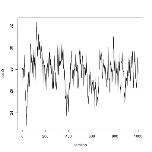
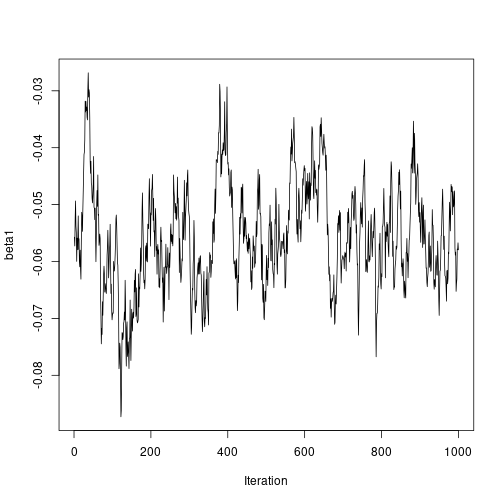
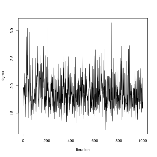
One method for reducing the autocorrelation in the sampling chains for regression parameters is to mean centre the covariate(s); this works because it reduces any dependence between the regression intercept and slope(s). Do this for the current example, noting that you will need to make a correction on the estimate of the regression intercept afterwards.
Solution
# Mean-centre the x covariate
DataC <- Data
meanx <- mean(DataC$x)
DataC$x <- DataC$x - meanx

# Bayesian Linear Regression using a Gibbs Sampler

# Set the number of iterations of the Gibbs Sampler - including how many to
# discard as the burn-in
m.burnin <- 500
m.keep <- 1000
m <- m.burnin + m.keep

# Obtain the samples
results2 <- gibbs_sample(DataC, 1, 1, 1, m, 1, 1, 0, 0.0001, 0, 0.0001)
# Remove the burn-in
results2 <- results2[-(1:m.burnin), ]

# Correct the effect of the mean-centering on the intercept
results2$beta0 <- results2$beta0 - meanx * results2$beta1

# Add variance and standard deviation columns
results2$Variance <- 1 / results2$tau
results2$StdDev <- sqrt(results2$Variance)
# Estimates are the column means
apply(results2[, -1], 2, mean)
## beta0 beta1 tau Variance StdDev ## 27.7619863 -0.0554732 0.3055647 3.5419578 1.8627159# Also look at uncertainty apply(results2[, -1], 2, sd)## beta0 beta1 tau Variance StdDev ## 1.339327429 0.008712278 0.084838193 1.070089030 0.268923052## beta0 beta1 tau Variance StdDev ## 2.5% 25.16694 -0.07283719 0.1603452 2.002122 1.414964 ## 97.5% 30.36258 -0.03852308 0.4994701 6.236545 2.497308# Kernel density plots for beta0, beta1 and the residual standard # deviation plot(density(results2$beta0, bw = 0.5), main = "Posterior density for beta0")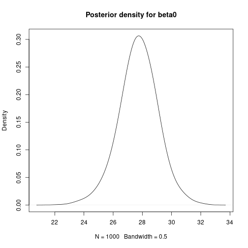 plot of chunk unnamed-chunk-7
 plot of chunk unnamed-chunk-7
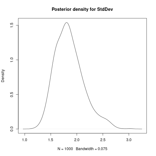 plot of chunk unnamed-chunk-7
# Plot sampled series ts.plot(results2$beta0, ylab = "beta0", xlab = "Iteration")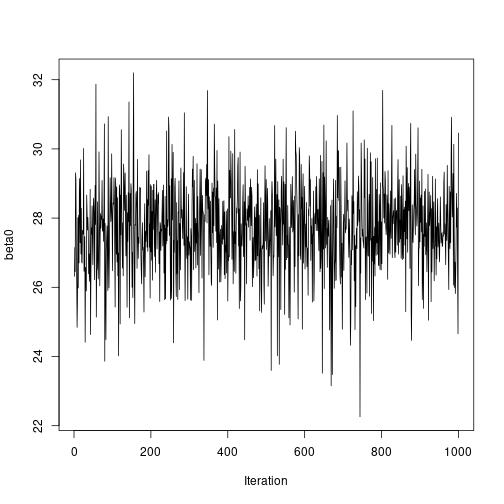 plot of chunk unnamed-chunk-7
ts.plot(results2$beta1, ylab = "beta1", xlab = "Iteration")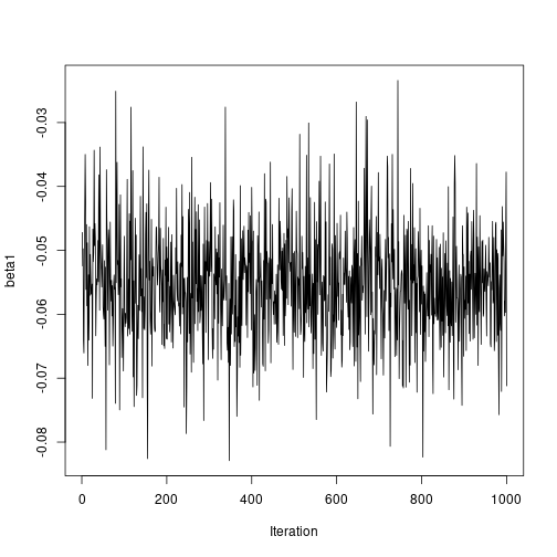 plot of chunk unnamed-chunk-7
ts.plot(results2$StdDev, ylab = "sigma", xlab = "Iteration")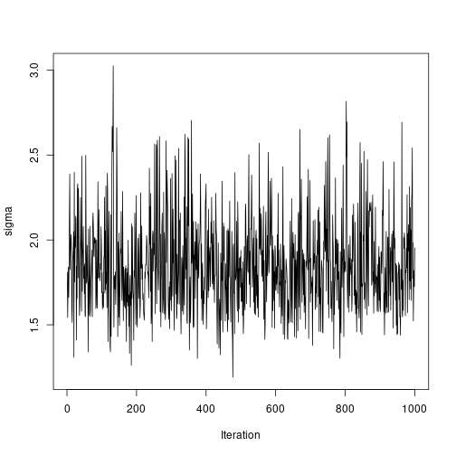 plot of chunk unnamed-chunk-7
INLA
INLA (https://www.r-inla.org/) is based on producing
(accurate) approximations to the marginal posterior distributions of the
model parameters. Although this can be enough most of the time, making
multivariate inference with INLA can be difficult or
impossible. However, in many cases this is not needed and
INLA can fit some classes of models in a fraction of the
time it takes with MCMC.
We can obtain Bayesian model fits without using MCMC with the INLA
software, implemented in R via the INLA package. If you do
not have this package installed already, as it is not on CRAN you will
need to install it via
install.packages(
  "INLA",
  repos = c(getOption("repos"), INLA="https://inla.r-inla-download.org/R/stable"),
  dep=TRUE
)
After this, the package can be loaded into R:
library(INLA)Example: Fake News
This section is included here as a reminder, as we are going to
reanalyse this data set using INLA.
The fake_news data set in the bayesrules
package in R contains information about 150 news articles,
some real news and some fake news.
In this example, we will look at trying to predict whether an article of news is fake or not given three explanatory variables.
We can use the following code to extract the variables we want from the data set:
library(bayesrules)
fakenews <- fake_news[,c("type","title_has_excl","title_words","negative")]
The response variable type takes values
fake or real, which should be
self-explanatory. The three explanatory variables are:
title_has_excl, whether or not the article contains an exclamation mark (valuesTRUEorFALSE);title_words, the number of words in the title (a positive integer); andnegative, a sentiment rating, recorded on a continuous scale.
In the exercise to follow, we will examine whether the chance of an article being fake news is related to the three covariates here.
Note that the variable title_has_excl will need to be
either replaced by or converted to a factor, for example
fakenews$titlehasexcl <- as.factor(fakenews$title_has_excl)Functions summary and confint produce a
summary (including parameter estimates etc) and confidence intervals for
the parameters, respectively.
Finally, we create a new version of the response variable of type logical:
fakenews$typeFAKE <- fakenews$type == "fake"Exercises
-
Perform an exploratory assessment of the fake news data set, in particular looking at the possible relationships between the explanatory variables and the fake/real response variable
typeFAKE. You may wish to use the R functionboxplot()here.Solution
# Is there a link between the fakeness and whether the title has an exclamation mark?
table(fakenews$title_has_excl, fakenews$typeFAKE)
## ## FALSE TRUE ## FALSE 88 44 ## TRUE 2 16# For the quantitative variables, look at boxplots on fake vs real boxplot(fakenews$title_words ~ fakenews$typeFAKE)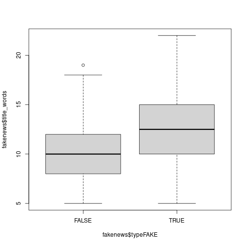 plot of chunk unnamed-chunk-13
boxplot(fakenews$negative ~ fakenews$typeFAKE)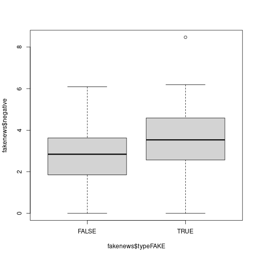 plot of chunk unnamed-chunk-13
 -
Fit the Bayesian model without MCMC using
INLA; note that the summary output provides credible intervals for each parameter to help us make inference. Also, inINLAa Binomial response needs to be entered as type integer, so we need another conversion:fakenews$typeFAKE.int <- as.integer(fakenews$typeFAKE)Solution
# Fit model - note similarity with bayesx syntax
inla.output <- inla(formula = typeFAKE.int ~ titlehasexcl + title_words + negative,
                    data = fakenews,
                    family = "binomial")
# Summarise output
summary(inla.output)
## Time used: ## Pre = 0.274, Running = 0.172, Post = 0.00536, Total = 0.452 ## Fixed effects: ## mean sd 0.025quant 0.5quant 0.975quant mode kld ## (Intercept) -3.016 0.761 -4.507 -3.016 -1.525 -3.016 0 ## titlehasexclTRUE 2.680 0.791 1.131 2.680 4.230 2.680 0 ## title_words 0.116 0.058 0.002 0.116 0.230 0.116 0 ## negative 0.328 0.154 0.027 0.328 0.629 0.328 0 ## ## Marginal log-Likelihood: -100.78 ## is computed ## Posterior summaries for the linear predictor and the fitted values are computed ## (Posterior marginals needs also 'control.compute=list(return.marginals.predictor=TRUE)') -
Fit a non-Bayesian model using
glm()for comparison. How do the model fits compare?Solution
# Fit model - note similarity with bayesx syntax
glm.output <- glm(formula = typeFAKE ~ titlehasexcl + title_words + negative,
                  data = fakenews,
                  family = "binomial")
# Summarise output
summary(glm.output)
## ## Call: ## glm(formula = typeFAKE ~ titlehasexcl + title_words + negative, ## family = "binomial", data = fakenews) ## ## Coefficients: ## Estimate Std. Error z value Pr(>|z|) ## (Intercept) -2.91516 0.76096 -3.831 0.000128 *** ## titlehasexclTRUE 2.44156 0.79103 3.087 0.002025 ** ## title_words 0.11164 0.05801 1.925 0.054278 . ## negative 0.31527 0.15371 2.051 0.040266 * ## --- ## Signif. codes: 0 '***' 0.001 '**' 0.01 '*' 0.05 '.' 0.1 ' ' 1 ## ## (Dispersion parameter for binomial family taken to be 1) ## ## Null deviance: 201.90 on 149 degrees of freedom ## Residual deviance: 169.36 on 146 degrees of freedom ## AIC: 177.36 ## ## Number of Fisher Scoring iterations: 4# Perform ANOVA on each variable in turn drop1(glm.output,test="Chisq")## Single term deletions ## ## Model: ## typeFAKE ~ titlehasexcl + title_words + negative ## Df Deviance AIC LRT Pr(>Chi) ## <none> 169.36 177.36 ## titlehasexcl 1 183.51 189.51 14.1519 0.0001686 *** ## title_words 1 173.17 179.17 3.8099 0.0509518 . ## negative 1 173.79 179.79 4.4298 0.0353162 * ## --- ## Signif. codes: 0 '***' 0.001 '**' 0.01 '*' 0.05 '.' 0.1 ' ' 1
Example: Emergency Room Complaints
This section is included here as a reminder, as we are going to
reanalyse this data set using INLA.
For this example we will use the esdcomp data set, which
is available in the faraway package. This data set records
complaints about emergency room doctors. In particular, data was
recorded on 44 doctors working in an emergency service at a hospital to
study the factors affecting the number of complaints received.
The response variable that we will use is complaints, an
integer count of the number of complaints received. It is expected that
the number of complaints will scale by the number of visits (contained
in the visits column), so we are modelling the rate of
complaints per visit - thus we will need to include a new variable
log.visits as an offset.
The three explanatory variables we will use in the analysis are:
residency, whether or not the doctor is still in residency training (valuesNorY);gender, the gender of the doctor (valuesForM); andrevenue, dollars per hour earned by the doctor, recorded as an integer.
Our simple aim here is to assess whether the seniority, gender or income of the doctor is linked with the rate of complaints against that doctor.
We can use the following code to extract the data we want without having to load the whole package:
esdcomp <- faraway::esdcompFitting Bayesian Poisson Regression Models
Again we can use INLA to fit this form of Bayesian
generalised linear model.
If not loaded already, the package must be loaded into R:
As noted above we need to include an offset in this analysis; since
for a Poisson GLM we will be using a log() link function by default, we
must compute the log of the number of visits and include that in the
data set esdcomp:
esdcomp$log.visits <- log(esdcomp$visits)The offset term in the model is then written
offset(log.visits)
Exercises
-
Perform an exploratory assessment of the emergency room complaints data set, particularly how the response variable
complaintsvaries with the proposed explanatory variables relative to the number of visits. To do this, create another variable which is the ratio ofcomplaintstovisits.Solution
# Compute the ratio esdcomp$ratio <- esdcomp$complaints / esdcomp$visits # Plot the link with revenue plot(esdcomp$revenue,esdcomp$ratio)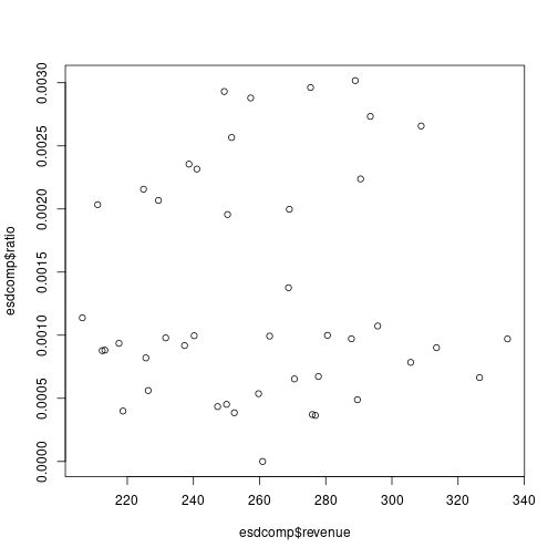 plot of chunk unnamed-chunk-20
# Use boxplots against residency and gender boxplot(esdcomp$ratio ~ esdcomp$residency)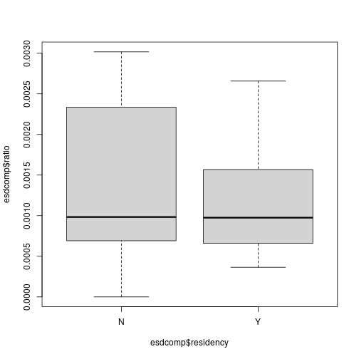 plot of chunk unnamed-chunk-20
boxplot(esdcomp$ratio ~ esdcomp$gender)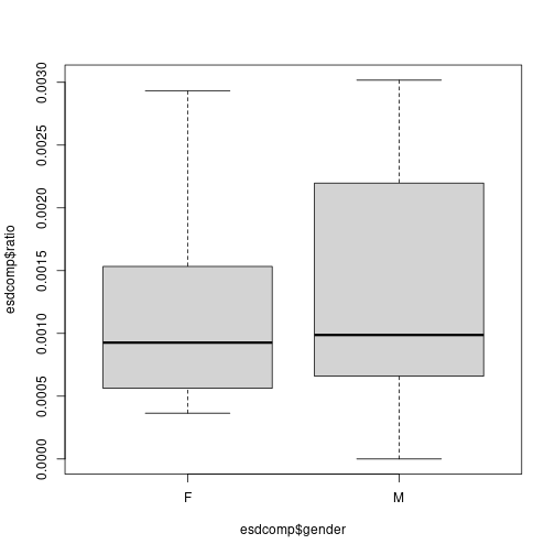 plot of chunk unnamed-chunk-20
 -
Fit the Bayesian model without MCMC using
INLA; note that the summary output provides credible intervals for each parameter to help us make inference.Solution
# Fit model - note similarity with bayesx syntax
inla.output <- inla(formula = complaints ~ offset(log.visits) + residency + gender + revenue,
                    data = esdcomp,
                    family = "poisson")
# Summarise output
summary(inla.output)
## Time used: ## Pre = 0.129, Running = 0.145, Post = 0.061, Total = 0.335 ## Fixed effects: ## mean sd 0.025quant 0.5quant 0.975quant mode kld ## (Intercept) -7.171 0.688 -8.520 -7.171 -5.822 -7.171 0 ## residencyY -0.354 0.191 -0.728 -0.354 0.021 -0.354 0 ## genderM 0.139 0.214 -0.281 0.139 0.559 0.139 0 ## revenue 0.002 0.003 -0.003 0.002 0.008 0.002 0 ## ## Marginal log-Likelihood: -111.90 ## is computed ## Posterior summaries for the linear predictor and the fitted values are computed ## (Posterior marginals needs also 'control.compute=list(return.marginals.predictor=TRUE)') -
Fit a non-Bayesian model using
glm()for comparison. How do the model fits compare?Solution
# Fit model - note similarity with bayesx syntax
esdcomp$log.visits <- log(esdcomp$visits)
glm.output <- glm(formula = complaints ~ offset(log.visits) + residency + gender + revenue,
                  data = esdcomp,
                  family = "poisson")
# Summarise output
summary(glm.output)
## ## Call: ## glm(formula = complaints ~ offset(log.visits) + residency + gender + ## revenue, family = "poisson", data = esdcomp) ## ## Coefficients: ## Estimate Std. Error z value Pr(>|z|) ## (Intercept) -7.157087 0.688148 -10.401 <2e-16 *** ## residencyY -0.350610 0.191077 -1.835 0.0665 . ## genderM 0.128995 0.214323 0.602 0.5473 ## revenue 0.002362 0.002798 0.844 0.3986 ## --- ## Signif. codes: 0 '***' 0.001 '**' 0.01 '*' 0.05 '.' 0.1 ' ' 1 ## ## (Dispersion parameter for poisson family taken to be 1) ## ## Null deviance: 63.435 on 43 degrees of freedom ## Residual deviance: 58.698 on 40 degrees of freedom ## AIC: 189.48 ## ## Number of Fisher Scoring iterations: 5# Perform ANOVA on each variable in turn drop1(glm.output, test = "Chisq")## Single term deletions ## ## Model: ## complaints ~ offset(log.visits) + residency + gender + revenue ## Df Deviance AIC LRT Pr(>Chi) ## <none> 58.698 189.48 ## residency 1 62.128 190.91 3.4303 0.06401 . ## gender 1 59.067 187.85 0.3689 0.54361 ## revenue 1 59.407 188.19 0.7093 0.39969 ## --- ## Signif. codes: 0 '***' 0.001 '**' 0.01 '*' 0.05 '.' 0.1 ' ' 1
Bayesian Hierarchical Modelling
These two final sections simply reproduce Practical 7, but using
INLA rather than BayesX.
Linear Mixed Models
Linear mixed models were defined in the lecture as follows:
Here, represents observation in group , is a vector of covariates with coefficients , i.i.d. random effects and a Gaussian error term. The distribution of the random effects is Gaussian with zero mean and precision .
Multilevel Modelling
Multilevel models are a particular type of mixed-effects models in which observations are nested within groups, so that group effects are modelled using random effects. A typical example is that of students nested within classes.
For the next example, the nlschools data set (in package
MASS) will be used. This data set records data about
students’ performance (in particular, about a language score test) and
other variables. The variables in this data set are:
lang, language score test.IQ, verbal IQ.class, class ID.GS, class size as number of eighth-grade pupils recorded in the class.SES, social-economic status of pupil’s family.COMB, whether the pupils are taught in the multi-grade class with 7th-grade students.
The data set can be loaded and summarised as follows:
##       lang             IQ            class            GS             SES        COMB
##  Min.   : 9.00   Min.   : 4.00   15580  :  33   Min.   :10.00   Min.   :10.00   0:1658
##  1st Qu.:35.00   1st Qu.:10.50   5480   :  31   1st Qu.:23.00   1st Qu.:20.00   1: 629
##  Median :42.00   Median :12.00   15980  :  31   Median :27.00   Median :27.00
##  Mean   :40.93   Mean   :11.83   16180  :  31   Mean   :26.51   Mean   :27.81
##  3rd Qu.:48.00   3rd Qu.:13.00   18380  :  31   3rd Qu.:31.00   3rd Qu.:35.00
##  Max.   :58.00   Max.   :18.00   5580   :  30   Max.   :39.00   Max.   :50.00
##                                  (Other):2100
The model to fit will take lang as the response variable
and include IQ, GS, SES and
COMB as covariates (i.e., fixed effects). This model can
easily be fit with INLA as follows:
## Time used:
##     Pre = 0.13, Running = 0.163, Post = 0.0111, Total = 0.305
## Fixed effects:
##               mean    sd 0.025quant 0.5quant 0.975quant   mode kld
## (Intercept)  9.685 1.070      7.586    9.685     11.784  9.685   0
## IQ           2.391 0.074      2.246    2.391      2.536  2.391   0
## GS          -0.026 0.025     -0.076   -0.026      0.024 -0.026   0
## SES          0.148 0.014      0.120    0.148      0.175  0.148   0
## COMB1       -1.684 0.325     -2.322   -1.684     -1.047 -1.684   0
##
## Model hyperparameters:
##                                          mean    sd 0.025quant 0.5quant 0.975quant  mode
## Precision for the Gaussian observations 0.021 0.001       0.02    0.021      0.022 0.021
##
## Marginal log-Likelihood:  -7713.44
##  is computed
## Posterior summaries for the linear predictor and the fitted values are computed
## (Posterior marginals needs also 'control.compute=list(return.marginals.predictor=TRUE)')
Note that the previous model only includes fixed effects. The data
set includes class as the class ID to which each student
belongs. Class effects can have an impact on the performance of the
students, with students in the same class performing similarly in the
language test.
Very conveniently, INLA can include random effects in
the model by adding a term in the right hand side of the formula that
defined the model. Specifically, the term to add is
f(class, model = "iid") (see code below for the full
model). This will create a random effect indexed over variable
class and which is of type iid, i.e., the
random effects are independent and identically distributed using a
normal distribution with zero mean and precision
.
Before fitting the model, the between-class variability can be explored by means of boxplots:
boxplot(lang ~ class, data = nlschools, las = 2)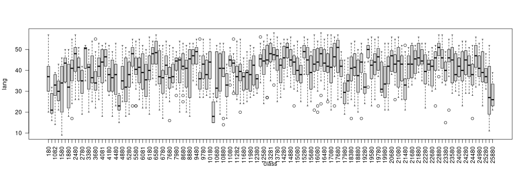
The code to fit the model with random effects is:
## Time used:
##     Pre = 0.814, Running = 0.19, Post = 0.0219, Total = 1.03
## Fixed effects:
##               mean    sd 0.025quant 0.5quant 0.975quant   mode kld
## (Intercept) 10.626 1.495      7.698   10.624     13.565 10.624   0
## IQ           2.248 0.072      2.108    2.248      2.388  2.248   0
## GS          -0.016 0.047     -0.109   -0.016      0.078 -0.016   0
## SES          0.165 0.015      0.136    0.165      0.194  0.165   0
## COMB1       -2.017 0.598     -3.193   -2.016     -0.847 -2.016   0
##
## Random effects:
##   Name     Model
##     class IID model
##
## Model hyperparameters:
##                                          mean    sd 0.025quant 0.5quant 0.975quant  mode
## Precision for the Gaussian observations 0.025 0.001      0.024    0.025      0.027 0.025
## Precision for class                     0.122 0.020      0.087    0.121      0.167 0.118
##
## Marginal log-Likelihood:  -7613.01
##  is computed
## Posterior summaries for the linear predictor and the fitted values are computed
## (Posterior marginals needs also 'control.compute=list(return.marginals.predictor=TRUE)')
Generalised Linear Mixed Models
Mixed effects models can also be considered within the context of generalised linear models. In this case, the linear predictor of observation , , can be defined as
Compared to the previous setting of linear mixed effects models, note that now the distribution of the response could be other than Gaussian and that observations are not necessarily nested within groups.
Poisson regression
In this practical we will use the North Carolina Sudden Infant Death
Syndrome (SIDS) data set. It is available in the spData
package and it can be loaded using:
##     CNTY.ID         BIR74           SID74          NWBIR74           BIR79           SID79
##  Min.   :1825   Min.   :  248   Min.   : 0.00   Min.   :   1.0   Min.   :  319   Min.   : 0.00
##  1st Qu.:1902   1st Qu.: 1077   1st Qu.: 2.00   1st Qu.: 190.0   1st Qu.: 1336   1st Qu.: 2.00
##  Median :1982   Median : 2180   Median : 4.00   Median : 697.5   Median : 2636   Median : 5.00
##  Mean   :1986   Mean   : 3300   Mean   : 6.67   Mean   :1051.0   Mean   : 4224   Mean   : 8.36
##  3rd Qu.:2067   3rd Qu.: 3936   3rd Qu.: 8.25   3rd Qu.:1168.5   3rd Qu.: 4889   3rd Qu.:10.25
##  Max.   :2241   Max.   :21588   Max.   :44.00   Max.   :8027.0   Max.   :30757   Max.   :57.00
##     NWBIR79             east           north             x                 y
##  Min.   :    3.0   Min.   : 19.0   Min.   :  6.0   Min.   :-328.04   Min.   :3757
##  1st Qu.:  250.5   1st Qu.:178.8   1st Qu.: 97.0   1st Qu.: -60.55   1st Qu.:3920
##  Median :  874.5   Median :285.0   Median :125.5   Median : 114.38   Median :3963
##  Mean   : 1352.8   Mean   :271.3   Mean   :122.1   Mean   :  91.46   Mean   :3953
##  3rd Qu.: 1406.8   3rd Qu.:361.2   3rd Qu.:151.5   3rd Qu.: 240.03   3rd Qu.:4000
##  Max.   :11631.0   Max.   :482.0   Max.   :182.0   Max.   : 439.65   Max.   :4060
##       lon              lat             L.id           M.id
##  Min.   :-84.08   Min.   :33.92   Min.   :1.00   Min.   :1.00
##  1st Qu.:-81.20   1st Qu.:35.26   1st Qu.:1.00   1st Qu.:2.00
##  Median :-79.26   Median :35.68   Median :2.00   Median :3.00
##  Mean   :-79.51   Mean   :35.62   Mean   :2.12   Mean   :2.67
##  3rd Qu.:-77.87   3rd Qu.:36.05   3rd Qu.:3.00   3rd Qu.:3.25
##  Max.   :-75.67   Max.   :36.52   Max.   :4.00   Max.   :4.00
A full description of the data set is provided in the associated
manual page (check with ?nc.sids) but in this practical we
will only consider these variables:
BIR74, number of births (1974-78).SID74, number of SID deaths (1974-78).NWBIR74, number of non-white births (1974-78).
These variables are measured at the county level in North Carolina, of which there are 100.
Because SID74 records the number of SID deaths, the
model is Poisson:
Here, represents the number of cases in county and the mean. In addition, mean will be written as , where is the expected number of cases and the relative risk in county .
The relative risk is often modelled, on the log-scale, to be equal to a linear predictor:
The expected number of cases is computed by multiplying the number of births in county to the overall mortality rate
where represents the total number of births in country . Hence, the expected number of cases in county is .
# Overall mortality rate
r74 <- sum(nc.sids$SID74) / sum(nc.sids$BIR74)
# Expected cases
nc.sids$EXP74 <- r74 * nc.sids$BIR74
A common measure of relative risk is the standardised mortality ratio ():
nc.sids$SMR74 <- nc.sids$SID74 / nc.sids$EXP74A summary of the SMR can be obtained:
hist(nc.sids$SMR, xlab = "SMR")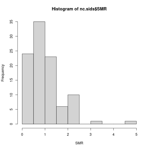
Values above 1 indicate that the county has more observed deaths than expected and that there might be an increased risk in the area.
As a covariate, we will compute the proportion of non-white births:
nc.sids$NWPROP74 <- nc.sids$NWBIR74/ nc.sids$BIR74There is a clear relationship between the SMR and the proportion of non-white births in a county:
plot(nc.sids$NWPROP74, nc.sids$SMR74)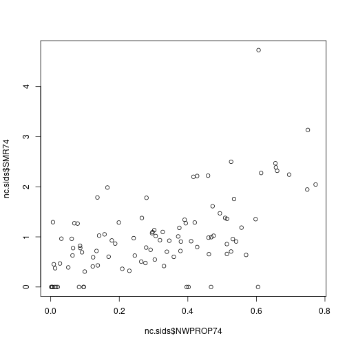
# Correlation
cor(nc.sids$NWPROP74, nc.sids$SMR74)
## [1] 0.5793901A simple Poisson regression can be fit by using the following code:
m1nc <- inla(
  SID74 ~ 1 + NWPROP74,
  family = "poisson",
  E = nc.sids$EXP74,
  data = nc.sids
)
summary(m1nc)
## Time used:
## Pre = 0.314, Running = 0.148, Post = 0.00488, Total = 0.467
## Fixed effects:
## mean sd 0.025quant 0.5quant 0.975quant mode kld
## (Intercept) -0.647 0.090 -0.824 -0.647 -0.471 -0.647 0
## NWPROP74 1.867 0.217 1.441 1.867 2.293 1.867 0
##
## Marginal log-Likelihood: -226.13
## is computed
## Posterior summaries for the linear predictor and the fitted values are computed
## (Posterior marginals needs also 'control.compute=list(return.marginals.predictor=TRUE)')Random effects can also be included to account for intrinsic differences between the counties:
# Index for random effects
nc.sids$ID <- seq_len(nrow(nc.sids))

# Model WITH covariate
m2nc <- inla(
  SID74 ~  1 + NWPROP74 + f(ID, model = "iid"),
  family = "poisson",
  E = nc.sids$EXP74,
  data = as.data.frame(nc.sids)
)

summary(m2nc)
## Time used:
## Pre = 0.138, Running = 0.157, Post = 0.00974, Total = 0.305
## Fixed effects:
## mean sd 0.025quant 0.5quant 0.975quant mode kld
## (Intercept) -0.650 0.104 -0.856 -0.649 -0.446 -0.649 0
## NWPROP74 1.883 0.254 1.386 1.882 2.385 1.882 0
##
## Random effects:
## Name Model
## ID IID model
##
## Model hyperparameters:
## mean sd 0.025quant 0.5quant 0.975quant mode
## Precision for ID 89.43 142.78 9.45 28.92 273.93 15.69
##
## Marginal log-Likelihood: -227.82
## is computed
## Posterior summaries for the linear predictor and the fitted values are computed
## (Posterior marginals needs also 'control.compute=list(return.marginals.predictor=TRUE)')The role of the covariate can be explored by fitting a model without it:
# Model WITHOUT covariate
m3nc <- inla(
  SID74 ~  1 + f(ID, model = "iid"),
  family = "poisson",
  E = nc.sids$EXP74,
  data = as.data.frame(nc.sids)
)

summary(m3nc)
## Time used:
## Pre = 0.145, Running = 0.166, Post = 0.00903, Total = 0.32
## Fixed effects:
## mean sd 0.025quant 0.5quant 0.975quant mode kld
## (Intercept) -0.029 0.063 -0.156 -0.028 0.091 -0.028 0
##
## Random effects:
## Name Model
## ID IID model
##
## Model hyperparameters:
## mean sd 0.025quant 0.5quant 0.975quant mode
## Precision for ID 7.26 2.57 3.79 6.77 13.55 6.01
##
## Marginal log-Likelihood: -245.52
## is computed
## Posterior summaries for the linear predictor and the fitted values are computed
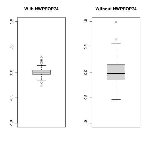
## (Posterior marginals needs also 'control.compute=list(return.marginals.predictor=TRUE)')Now, notice the decrease in the estimate of the precision of the random effects (i.e., the variance increases). This means that values of the random effects are now larger than in the previous case as the random effects pick some of the effect explained by the covariate.
oldpar <- par(mfrow = c(1, 2))
boxplot(m2nc$summary.random$ID$mean, ylim = c(-1, 1), main = "With NWPROP74")
boxplot(m3nc$summary.random$ID$mean, ylim = c(-1, 1), main = "Without NWPROP74")
par(oldpar)